During the telecommunication boom, Claude Shannon, in his seminal 1948 paper¹, posed a question that would revolutionise technology:
How can we quantify communication?
Shannon’s findings remain fundamental to expressing information quantification, storage, and communication. These insights made major contributions to the creation of technologies ranging from signal processing, data compression (e.g., Zip files and compact discs) to the Internet and artificial intelligence. More broadly, his work has significantly impacted diverse fields such as neurobiology, statistical physics and computer science (e.g, cybersecurity, cloud computing, and machine learning).
[Shannon’s paper is the]
Magna Carta of the Information Age
- Scientific American
This is the first article in a series that explores information quantification – an essential tool for data scientists. Its applications range from enhancing statistical analyses to serving as a go-to decision heuristic in cutting-edge machine learning algorithms.
Broadly speaking, quantifying information is assessing uncertainty, which may be phrased as: “how surprising is an outcome?”.
This article idea quickly grew into a series since I found this topic both fascinating and diverse. Most researchers, at one stage or another, come across commonly used metrics such as entropy, cross-entropy/KL-divergence and mutual-information. Diving into this topic I found that in order to fully appreciate these one needs to learn a bit about the basics which we cover in this first article.
By reading this series you will gain an intuition and tools to quantify:
- Bits/Nats – Unit measures of information.
- Self-Information – **** The amount of information in a specific event.
- Pointwise Mutual Information – The amount of information shared between two specific events.
- Entropy – The average amount of information of a variable’s outcome.
- Cross-entropy – The misalignment between two probability distributions (also expressed by its derivative KL-Divergence – a distance measure).
- Mutual Information – The co-dependency of two variables by their conditional probability distributions. It expresses the information gain of one variable given another.
No prior knowledge is required – just a basic understanding of probabilities.
I demonstrate using common statistics such as coin and dice 🎲 tosses as well as machine learning applications such as in supervised classification, feature selection, model monitoring and clustering assessment. As for real world applications I’ll discuss a case study of quantifying DNA diversity 🧬. Finally, for fun, I also apply to the popular brain twister commonly known as the Monty Hall problem 🚪🚪 🐐 .
Throughout I provide python code 🐍 , and try to keep formulas as intuitive as possible. If you have access to an integrated development environment (IDE) 🖥 you might want to plug 🔌 and play 🕹 around with the numbers to gain a better intuition.
This series is divided into four articles, each exploring a key aspect of Information Theory:
-
😲 Quantifying Surprise: 👈 👈 👈 YOU ARE HERE
In this opening article, you’ll learn how to quantify the “surprise” of an event using _self-informatio_n and understand its units of measurement, such as _bit_s and _nat_s. Mastering self-information is essential for building intuition about the subsequent concepts, as all later heuristics are derived from it. - 🤷 Quantifying Uncertainty: Building on self-information, this article shifts focus to the uncertainty – or “average surprise” – associated with a variable, known as entropy. We’ll dive into entropy’s wide-ranging applications, from Machine Learning and data analysis to solving fun puzzles, showcasing its adaptability.
- 📏 Quantifying Misalignment: Here, we’ll explore how to measure the distance between two probability distributions using entropy-based metrics like cross-entropy and KL-divergence. These measures are particularly valuable for tasks like comparing predicted versus true distributions, as in classification loss functions and other alignment-critical scenarios.
- 💸 Quantifying Gain: Expanding from single-variable measures, this article investigates the relationships between two. You’ll discover how to quantify the information gained about one variable (e.g, target Y) by knowing another (e.g., predictor X). Applications include assessing variable associations, feature selection, and evaluating clustering performance.
Each article is crafted to stand alone while offering cross-references for deeper exploration. Together, they provide a practical, data-driven introduction to information theory, tailored for data scientists, analysts and machine learning practitioners.
Disclaimer: Unless otherwise mentioned the formulas analysed are for categorical variables with c≥2 classes (2 meaning binary). Continuous variables will be addressed in a separate article.
🚧 Articles (3) and (4) are currently under construction. I will share links once available. Follow me to be notified 🚧
Quantifying Surprise with Self-Information
Self-information is considered the building block of information quantification.
It is a way of quantifying the amount of “surprise” of a specific outcome.
Formally self-information, or also referred to as Shannon Information or information content, quantifies the surprise of an event x occurring based on its probability, p(x). Here we denote it as hₓ:

The units of measure are called bits. One bit (binary digit) is the amount of information for an event x that has probability of p(x)=½. Let’s plug in to verify: hₓ=-log₂(½)= log₂(2)=1 bit.
This heuristic serves as an alternative to probabilities, odds and log-odds, with certain mathematical properties which are advantageous for information theory. We discuss these below when learning about Shannon’s axioms behind this choice.
It’s always informative to explore how an equation behaves with a graph:
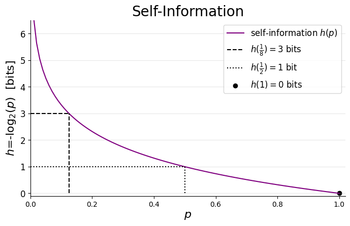
To deepen our understanding of self-information, we’ll use this graph to explore the said axioms that justify its logarithmic formulation. Along the way, we’ll also build intuition about key features of this heuristic.
To emphasise the logarithmic nature of self-information, I’ve highlighted three points of interest on the graph:
- At p=1 an event is guaranteed, yielding no surprise and hence zero bits of information (zero bits). A useful analogy is a trick coin (where both sides show HEAD).
- Reducing the probability by a factor of two (p=½) increases the information to _hₓ=_1 bit. This, of course, is the case of a fair coin.
- Further reducing it by a factor of four results in hₓ(p=⅛)=3 bits.
If you are interested in coding the graph here is a python script:
To summarise this section:
Self-Information hₓ=-log₂(p(x)) quantifies the amount of “surprise” of a specific outcome x.
Three Axioms
Referencing prior work by Ralph Hartley, Shannon chose -log₂(p) as a manner to meet three axioms. We’ll use the equation and graph to examine how these are manifested:
-
An event with probability 100% is not surprising and hence does not yield any information.
In the trick coin case this is evident by p(x)=1 yielding hₓ=0. -
Less probable events are more surprising and provide more information.
This is apparent by self-information decreasing monotonically with increasing probability. - The property of Additivity – the total self-information of two independent events equals the sum of individual contributions. This will be explored further in the upcoming fourth article on Mutual Information.
There are mathematical proofs (which are beyond the scope of this series) that show that only the log function adheres to all three².
The application of these axioms reveals several intriguing and practical properties of self-information:
Important properties :
- Minimum bound: The first axiom hₓ(p=1)=0 establishes that self-information is non-negative, with zero as its lower bound. This is highly practical for many applications.
- Monotonically decreasing: The second axiom ensures that self-information decreases monotonically with increasing probability.
- No Maximum bound: At the extreme where _p→_0, monotonicity leads to self-information growing without bound hₓ(_p→0) →_ ∞, a feature that requires careful consideration in some contexts. However, when averaging self-information – as we will later see in the calculation of entropy – probabilities act as weights, effectively limiting the contribution of highly improbable events to the overall average. This relationship will become clearer when we explore entropy in detail.
It is useful to understand the close relationship to log-odds. To do so we define p(x) as the probability of event x to happen and p(¬x)=1-p(x) of it not to happen. log-odds(x) = log₂(p(x)/p(¬x))= h(¬x) – h(x).
The main takeaways from this section are
Axiom 1: An event with probability 100% is not surprising
Axiom 2: Less probable events are more surprising and, when they occur, provide more information.
Self information (1) monotonically decreases (2) with a minimum bound of zero and (3) no upper bound.
In the next two sections we further discuss units of measure and choice of normalisation.
Information Units of Measure
Bits or Shannons?
A bit, as mentioned, represents the amount of information associated with an event that has a 50% probability of occurring.
The term is also sometimes referred to as a Shannon, a naming convention proposed by mathematician and physicist David MacKay to avoid confusion with the term ‘bit’ in the context of digital processing and storage.
After some deliberation, I decided to use ‘bit’ throughout this series for several reasons:
- This series focuses on quantifying information, not on digital processing or storage, so ambiguity is minimal.
- Shannon himself, encouraged by mathematician and statistician John Tukey, used the term ‘bit’ in his landmark paper.
- ‘Bit’ is the standard term in much of the literature on information theory.
- For convenience – it’s more concise
Normalisation: Log Base 2 vs. Natural
Throughout this series we use base 2 for logarithms, reflecting the intuitive notion of a 50% chance of an event as a fundamental unit of information.
An alternative commonly used in machine learning is the natural logarithm, which introduces a different unit of measure called nats (short for natural units of information). One nat corresponds to the information gained from an event occurring with a probability of 1/e where e is Euler’s number (≈2.71828). In other words, 1 nat = -ln(p=(1/e)).
The relationship between bits (base 2) and nats (natural log) is as follows:
1 bit = ln(2) nats ≈ 0.693 nats.
Think of it as similar to a monetary current exchange or converting centimeters to inches.
In his seminal publication Shanon explained that the optimal choice of base depends on the specific system being analysed (paraphrased slightly from his original work):
- “A device with two stable positions […] can store one bit of information” (bit as in binary digit).
- “A digit wheel on a desk computing machine that has ten stable positions […] has a storage capacity of one decimal digit.”³
- “In analytical work where integration and differentiation are involved the base e is sometimes useful. The resulting units of information will be called natural units.“
Key aspects of machine learning, such as popular loss functions, often rely on integrals and derivatives. The natural logarithm is a practical choice in these contexts because it can be derived and integrated without introducing additional constants. This likely explains why the machine learning community frequently uses nats as the unit of information – it simplifies the mathematics by avoiding the need to account for factors like ln(2).
As shown earlier, I personally find base 2 more intuitive for interpretation. In cases where normalisation to another base is more convenient, I will make an effort to explain the reasoning behind the choice.
To summarise this section of units of measure:
bit = amount of information to distinguish between two equally likely outcomes.
Now that we are familiar with self-information and its unit of measure let’s examine a few use cases.
Quantifying Event Information with Coins and Dice
In this section, we’ll explore examples to help internalise the self-information axioms and key features demonstrated in the graph. Gaining a solid understanding of self-information is essential for grasping its derivatives, such as entropy, cross-entropy (or KL divergence), and mutual information – all of which are averages over self-information.
The examples are designed to be simple, approachable, and lighthearted, accompanied by practical Python code to help you experiment and build intuition.
Note: If you feel comfortable with self-information, feel free to skip these examples and go straight to the Quantifying Uncertainty article.

To further explore the self-information and bits, I find analogies like coin flips and dice rolls particularly effective, as they are often useful analogies for real-world phenomena. Formally, these can be described as multinomial trials with n=1 trial. Specifically:
- A coin flip is a Bernoulli trial, where there are c=2 possible outcomes (e.g., heads or tails).
- Rolling a die represents a categorical trial, where c≥3 outcomes are possible (e.g., rolling a six-sided or eight-sided die).
As a use case we’ll use simplistic weather reports limited to featuring sun 🌞 , rain 🌧 , and snow ⛄️.
Now, let’s flip some virtual coins 👍 and roll some funky-looking dice 🎲 …
Fair Coins and Dice

We’ll start with the simplest case of a fair coin (i.e, 50% chance for success/Heads or failure/Tails).
Imagine an area for which at any given day there is a 50:50 chance for sun or rain. We can write the probability of each event be: p(🌞 )=p(🌧 )=½.
As seen above, according the the self-information formulation, when 🌞 or 🌧 is reported we are provided with h(🌞 __ )=h(🌧 )=-log₂(½)=1 bit of information.
We will continue to build on this analogy later on, but for now let’s turn to a variable that has more than two outcomes (c≥3).
Before we address the standard six sided die, to simplify the maths and intuition, let’s assume an 8 sided one (_c=_8) as in Dungeons Dragons and other tabletop games. In this case each event (i.e, landing on each side) has a probability of p(🔲 ) = ⅛.
When a die lands on one side facing up, e.g, value 7️⃣, we are provided with h(🔲 =7️⃣)=-log₂(⅛)=3 bits of information.
For a standard six sided fair die: p(🔲 ) = ⅙ → an event yields __ h(🔲 )=-log₂(⅙)=2.58 bits.
Comparing the amount of information from the fair coin (1 bit), 6 sided die (2.58 bits) and 8 sided (3 bits) we identify the second axiom: The less probable an event is, the more surprising it is and the more information it yields.
Self information becomes even more interesting when probabilities are skewed to prefer certain events.
Loaded Coins and Dice

Let’s assume a region where p(🌞 ) = ¾ and p(🌧 )= ¼.
When rain is reported the amount of information conveyed is not 1 bit but rather h(🌧 )=-log₂(¼)=2 bits.
When sun is reported less information is conveyed: h(🌞 )=-log₂(¾)=0.41 bits.
As per the second axiom— a rarer event, like p(🌧 )=¼, reveals more information than a more likely one, like p(🌞 )=¾ – and vice versa.
To further drive this point let’s now assume a desert region where p(🌞 ) =99% and p(🌧 )= 1%.
If sunshine is reported – that is kind of expected – so nothing much is learnt (“nothing new under the sun” 🥁) and this is quantified as h(🌞 )=0.01 bits. If rain is reported, however, you can imagine being quite surprised. This is quantified as h(🌧 )=6.64 bits.
In the following python scripts you can examine all the above examples, and I encourage you to play with your own to get a feeling.
First let’s define the calculation and printout function:
import numpy as np

def print_events_self_information(probs):
    for ps in probs:
        print(f"Given distribution {ps}")
        for event in ps:
            if ps[event] != 0:
                self_information = -np.log2(ps[event]) #same as: -np.log(ps[event])/np.log(2)
                text_ = f'When `{event}` occurs {self_information:0.2f} bits of information is communicated'
                print(text_)
            else:
                print(f'a `{event}` event cannot happen p=0 ')
        print("=" * 20)
Next we’ll set a few example distributions of weather frequencies
# Setting multiple probability distributions (each sums to 100%)
# Fun fact - 🐍  💚  Emojis!
probs = [{'🌞   ': 0.5, '🌧   ': 0.5},   # half-half
        {'🌞   ': 0.75, '🌧   ': 0.25},  # more sun than rain
        {'🌞   ': 0.99, '🌧   ': 0.01} , # mostly sunshine
]

print_events_self_information(probs)
This yields printout
Given distribution {'🌞      ': 0.5, '🌧      ': 0.5}
When `🌞      ` occurs 1.00 bits of information is communicated
When `🌧      ` occurs 1.00 bits of information is communicated
====================
Given distribution {'🌞      ': 0.75, '🌧      ': 0.25}
When `🌞      ` occurs 0.42 bits of information is communicated
When `🌧      ` occurs 2.00 bits of information is communicated
====================
Given distribution {'🌞      ': 0.99, '🌧      ': 0.01}
When `🌞      ` occurs 0.01 bits of information is communicated
When `🌧      ` occurs 6.64 bits of information is communicated
Let’s examine a case of a loaded three sided die. E.g, information of a weather in an area that reports sun, rain and snow at uneven probabilities: p(🌞 ) = 0.2, p(🌧 )=0.7, p(⛄️)=0.1.
Running the following
print_events_self_information([{'🌞 ': 0.2, '🌧 ': 0.7, '⛄️': 0.1}])yields
Given distribution {'🌞  ': 0.2, '🌧  ': 0.7, '⛄️': 0.1}
When `🌞  ` occurs 2.32 bits of information is communicated
When `🌧  ` occurs 0.51 bits of information is communicated
When `⛄️` occurs 3.32 bits of information is communicated
What we saw for the binary case applies to higher dimensions.
To summarise – we clearly see the implications of the second axiom:
- When a highly expected event occurs – we do not learn much, the bit count is low.
- When an unexpected event occurs – we learn a lot, the bit count is high.
Event Information Summary
In this article we embarked on a journey into the foundational concepts of information theory, defining how to measure the surprise of an event. Notions introduced serve as the bedrock of many tools in information theory, from assessing data distributions to unraveling the inner workings of machine learning algorithms.
Through simple yet insightful examples like coin flips and dice rolls, we explored how self-information quantifies the unpredictability of specific outcomes. Expressed in bits, this measure encapsulates Shannon’s second axiom: rarer events convey more information.
While we’ve focused on the information content of specific events, this naturally leads to a broader question: what is the average amount of information associated with all possible outcomes of a variable?
In the next article, Quantifying Uncertainty, we build on the foundation of self-information and bits to explore entropy – the measure of average uncertainty. Far from being just a beautiful theoretical construct, it has practical applications in data analysis and machine learning, powering tasks like decision tree optimisation, estimating diversity and more.

Loved this post? ❤️🍕
💌 Follow me here, join me on LinkedIn or 🍕 buy me a pizza slice!
About This Series
Even though I have twenty years of experience in data analysis and predictive modelling I always felt quite uneasy about using concepts in information theory without truly understanding them.
The purpose of this series was to put me more at ease with concepts of information theory and hopefully provide for others the explanations I needed.
Check out my other articles which I wrote to better understand Causality and Bayesian Statistics:
Footnotes
¹ A Mathematical Theory of Communication, Claude E. Shannon, Bell System Technical Journal 1948.
It was later renamed to a book The Mathematical Theory of Communication in 1949.
[Shannon’s “A Mathematical Theory of Communication”] the blueprint for the digital era – Historian James Gleick
² See Wikipedia page on Information Content (i.e, self-information) for a detailed derivation that only the log function meets all three axioms.
³ The decimal-digit was later renamed to a hartley (symbol Hart), a ban or a dit. See Hartley (unit) Wikipedia page.
Credits
Unless otherwise noted, all images were created by the author.
Many thanks to Will Reynolds and Pascal Bugnion for their useful comments.