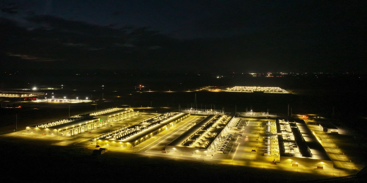
Your Gateway to Power, Energy, Datacenters, Bitcoin and AI

Dive into the latest industry updates, our exclusive Paperboy Newsletter, and curated insights designed to keep you informed. Stay ahead with minimal time spent.

Discover What Matters Most to You

Explore ONMINE’s curated content, from our Paperboy Newsletter to industry-specific insights tailored for energy, Bitcoin mining, and AI professionals.

AI

Lorem Ipsum is simply dummy text of the printing and typesetting industry.

Bitcoin:

Lorem Ipsum is simply dummy text of the printing and typesetting industry.

Datacenter:

Lorem Ipsum is simply dummy text of the printing and typesetting industry.

Energy:

Lorem Ipsum is simply dummy text of the printing and typesetting industry.

Shape
Discover What Matter Most to You

Featured Articles

Raizen Is Said to Hire JPMorgan for Argentina Energy Assets Sale

Brazil’s Raizen SA has begun to explore the sale of its oil refinery and network of gas stations in Argentina, according to people familiar with the matter. Raizen, a joint venture between oil supermajor Shell Plc and Brazilian conglomerate Cosan SA, has hired JPMorgan Chase & Co. to manage the sale, said the people, who asked not to be named discussing private matters. Press offices for Raizen and JPMorgan declined to comment.  The energy firm’s potential departure from Argentina would add to a growing list of multinational firms, including Exxon Mobil, HSBC Holdings Plc and Mercedes-Benz, that have chosen to sell operations in the country during the past year despite more investor optimism about President Javier Milei’s economic overhaul.  Brazil’s largest producer of ethanol fuel, Raizen is mulling divestments and slowing down expansions as higher borrowing costs of late in Brazil rattle its finances. Its Dock Sud oil refinery in Buenos Aires is Argentina’s oldest with a capacity of 100,000 barrels a day that only trails two facilities run by state-run oil company YPF SA. Raizen’s network of around 700 gas stations account for 18% of Argentina’s gasoline and diesel sales, second to YPF, which has more than half of the market. The fuel is branded as Shell. Raizen bought the assets for almost $1 billion in 2018 from Shell, which owned them outright, during Argentina’s last experiment with market-oriented reforms. The country then witnessed a period of big government from 2019 to 2023 before voting in libertarian Milei more than a year ago. He is on a crusade to deregulate the economy, in particular the energy and oil sectors. The divestment comes as Milei rips away controls on crude and fuel prices that were used to stem inflation. That was sometimes bad for refiners or drillers, depending on how

Read More »

Bonneville opts to join SPP’s Markets+ day-ahead market over CAISO alternative

Dive Brief: The Bonneville Power Administration plans to join the Southwest Power Pool’s Markets+ real-time and day-ahead market instead of a market being launched by the California Independent System Operator, BPA said in a draft policy released Wednesday. While the CAISO’s Extended Day-Ahead Market may offer greater financial benefits compared to Markets+, overall the SPP market is a better fit for BPA based on market design elements covering governance, resource adequacy, greenhouse gas accounting and congestion revenue, the federal power marketer said. Bonneville expects to make a final decision in May. The BPA’s draft decision sets the stage for the creation of two intertwined day-ahead markets in the West. “The idea that there’s some West-wide market ideal out there that we can get to today is just not something that is on the table,” Rachel Dibble, BPA power services vice president of bulk marketing, said at a press briefing Thursday. “Maybe someday, in future decades, there may be a point where we could merge into one market, but right now, there are many entities who support Markets+.” Dive Insight: The BPA’s decision will have a major effect on market development in the West. It sells wholesale power from federal hydroelectric dams in the Northwest, totaling about 22.4 GW. The federal power marketer also operates about 15,000 circuit miles of high-voltage transmission across the Northwest. The BPA mainly sells its power to cooperative and municipal utilities, and public power districts. In its draft decision, BPA rejected calls to wait for the West-Wide Governance Pathways Initiative to complete its effort to establish an independent governance framework for EDAM.  While a bill — SB 540 — was introduced in the California Legislature last month to implement the Pathways’ second phase, it “limits the availability of full operational administrative independence by requiring that the

Read More »

Trump extends tariff pause to all USMCA goods

The White House announced Thursday afternoon that it will suspend tariffs on all imports that are compliant with the United States-Mexico-Canada Agreement until April 2. The pause, which was extended to imports from Mexico that adhered to the USMCA earlier Thursday, will now also cover goods from Canada that meet the trade deal’s requirements. The move builds on Wednesday’s exemption for car imports from either country. “Today, President Donald J. Trump announced adjustments to tariffs imposed on imports from Canada and Mexico in recognition of the structure of the automotive supply chain that strives to bring production into America,” per a White House statement released Thursday. Roughly half of Mexico imports to the U.S. are USMCA compliant, while nearly 40% of those from Canada are, CNBC reported, citing a White House official. The U.S. is preparing to enact a universal reciprocal tariff policy on April 2, the day the pause ends. Trump and Mexico President Claudia Sheinbaum came to terms on a tariff pause on Thursday morning. The president said he made the decision “out of respect for” Sheinbaum while praising her cooperation in addressing fentanyl trafficking. “We’ll continue to work together, particularly on the topics of migration and safety that include reducing illegal crossing of fentanyl to the United States as well as weapons to Mexico,” Sheinbaum said in Spanish in a post on X.

Read More »

Data center supply, construction surged in 2024 amid AI boom

Dive Brief: Data center supply in major “primary” markets like Northern Virginia, Atlanta and Chicago surged 34% year-over-year in 2024 to 6,922.6 MW, with a further 6,350 MW under construction at year-end, CBRE said in a Feb. 26 report. The data center vacancy rate in primary markets fell to 1.9%, driving up the average asking rates for a 250-to-500-kilowatt requirement by 2.6% year-over-year to $184.06/kW, reflecting tight supply and robust demand for AI and cloud services, CBRE said in its North America Data Center Trends H2 2024 report. Volume-based discounts for larger tenants “have been significantly reduced or eliminated” due to rising demand for large, contiguous spaces, while data center operators grapple with elevated construction and equipment costs and “persistent shortages in critical materials like generators, chillers and transformers,” CBRE said. Dive Insight: Surging demand from organizations’ use of AI is driving the record data center development, CBRE says. The demand is giving AI-related occupiers increasing influence over data center development decisions like site selection, design and operational requirements. These occupiers are “prioritizing markets with scalable power capacity and advanced connectivity solutions,” the report says.  Demand is also showing up in pricing trends.  Last year was the third consecutive year of pricing increases for 250-to-500-kW slots in primary markets, CBRE said. Following steady single-digit annual declines from 2015 to 2021, average pricing rose 14.5% in 2022, 18.6% in 2023 and 12.6% in 2024. Robust tenant demand, healthy investor appetite for alternative real estate assets and recent interest rate declines are among the factors fueling an exponential increase in data center investment activity, CBRE said. Annual sales volumes reached $6.5 billion in 2024 as average sale prices increased year-over-year, reflecting “the growing scale of data center campuses,” CBRE said. Five transactions exceeded $400 million last year. Notable capital market developments included

Read More »

Oil Gains on Truce Hopes but Closes Week Lower

Oil’s one-day advance wasn’t enough to rescue prices from a seventh straight weekly decline as the prospect of a temporary truce in Ukraine capped on-again, off-again tariff news that upended global markets. West Texas Intermediate futures climbed by 0.7% Friday to settle above $67 a barrel after Bloomberg reported that Russia is open to a pause to fighting in Ukraine, raising the prospect of a resumption in Moscow’s crude exports. US President Donald Trump earlier pressured the two warring nations to hasten peace talks and the White House signaled that it may relax sanctions on Russian oil if there’s progress. Crude also found support from a weakening dollar and US plans to refill its strategic oil reserve, but still was down 3.9% on the week. The Biden administration’s farewell sanctions on Russia have snarled the nation’s crude trade in recent months, with total oil and natural gas revenue last month falling almost 19% from a year earlier, Bloomberg calculations showed. Russia’s oil-related taxes are a key source of financing its war against Ukraine. A potential reintroduction of Russian barrels to the market comes amid a gloomy period for the supply outlook, as OPEC+ forges ahead with a plan to start reviving idled output in April. Meanwhile, Trump’s trade policies have fanned concerns about reduced global energy demand. “You’re seeing some volatility as people try to interpret what they think is going to happen and what it’s going to mean, but the bottom line is Russia has been able to sell its oil,” said Amy Jaffe, director of New York University’s Energy, Climate Justice and Sustainability Lab. Trump signed orders on Thursday paring back tariffs on Mexico and Canada until April 2. That timing coincides with a date when the president is expected to start detailing plans for so-called reciprocal duties

Read More »

USA Won’t Hesitate on Russia and Iran Sanctions, Bessent Says

The US will not hesitate to go “all in” on sanctions on Russian energy if it helps lead to a ceasefire in the Ukraine war, Treasury Secretary Scott Bessent said Thursday. Sanctions on Russia “will be used explicitly and aggressively for immediate maximum impact” at President Donald Trump’s guidance, Bessent told an audience at the Economic Club of New York. The Trump administration is pressing Ukraine to come to the table for a ceasefire deal with Russia, and Bessent said additional sanctions on Russia could help give the US more leverage in the negotiations. Trump is ready to finalize an agreement that would give the US rights to help develop some of Ukraine’s natural resources if Ukrainian President Volodymyr Zelenskiy agrees to a tangible path for a truce and talks with Moscow, according to people familiar with the matter. Bessent criticized the Biden administration for not going harder on Russian energy sanctions for fear of driving up gas prices and asked what the point of “substantial US military and financial support over the past three years” was without matching sanctions. The US has paused military aid and some intelligence sharing with Ukraine in an effort to force the US ally to agree to negotiations with Russia over the end of the war. Bessent also said the US would ramp up sanctions on Iran, adding that the US will “shutdown” the country’s oil sector using “pre-determined benchmarks and timelines” and that “Making Iran broke again will mark the beginning of our updated sanctions policy.” The Treasury chief suggested that the US would work with “regional parties” that help Iran move its oil onto the market. One of those countries is likely to be Russia, which signaled earlier this week that it was willing to assist the US in talks with Iran on ending its nuclear

Read More »

Raizen Is Said to Hire JPMorgan for Argentina Energy Assets Sale

Brazil’s Raizen SA has begun to explore the sale of its oil refinery and network of gas stations in Argentina, according to people familiar with the matter. Raizen, a joint venture between oil supermajor Shell Plc and Brazilian conglomerate Cosan SA, has hired JPMorgan Chase & Co. to manage the sale, said the people, who asked not to be named discussing private matters. Press offices for Raizen and JPMorgan declined to comment.  The energy firm’s potential departure from Argentina would add to a growing list of multinational firms, including Exxon Mobil, HSBC Holdings Plc and Mercedes-Benz, that have chosen to sell operations in the country during the past year despite more investor optimism about President Javier Milei’s economic overhaul.  Brazil’s largest producer of ethanol fuel, Raizen is mulling divestments and slowing down expansions as higher borrowing costs of late in Brazil rattle its finances. Its Dock Sud oil refinery in Buenos Aires is Argentina’s oldest with a capacity of 100,000 barrels a day that only trails two facilities run by state-run oil company YPF SA. Raizen’s network of around 700 gas stations account for 18% of Argentina’s gasoline and diesel sales, second to YPF, which has more than half of the market. The fuel is branded as Shell. Raizen bought the assets for almost $1 billion in 2018 from Shell, which owned them outright, during Argentina’s last experiment with market-oriented reforms. The country then witnessed a period of big government from 2019 to 2023 before voting in libertarian Milei more than a year ago. He is on a crusade to deregulate the economy, in particular the energy and oil sectors. The divestment comes as Milei rips away controls on crude and fuel prices that were used to stem inflation. That was sometimes bad for refiners or drillers, depending on how

Read More »

Data center supply, construction surged in 2024 amid AI boom

Dive Brief: Data center supply in major “primary” markets like Northern Virginia, Atlanta and Chicago surged 34% year-over-year in 2024 to 6,922.6 MW, with a further 6,350 MW under construction at year-end, CBRE said in a Feb. 26 report. The data center vacancy rate in primary markets fell to 1.9%, driving up the average asking rates for a 250-to-500-kilowatt requirement by 2.6% year-over-year to $184.06/kW, reflecting tight supply and robust demand for AI and cloud services, CBRE said in its North America Data Center Trends H2 2024 report. Volume-based discounts for larger tenants “have been significantly reduced or eliminated” due to rising demand for large, contiguous spaces, while data center operators grapple with elevated construction and equipment costs and “persistent shortages in critical materials like generators, chillers and transformers,” CBRE said. Dive Insight: Surging demand from organizations’ use of AI is driving the record data center development, CBRE says. The demand is giving AI-related occupiers increasing influence over data center development decisions like site selection, design and operational requirements. These occupiers are “prioritizing markets with scalable power capacity and advanced connectivity solutions,” the report says.  Demand is also showing up in pricing trends.  Last year was the third consecutive year of pricing increases for 250-to-500-kW slots in primary markets, CBRE said. Following steady single-digit annual declines from 2015 to 2021, average pricing rose 14.5% in 2022, 18.6% in 2023 and 12.6% in 2024. Robust tenant demand, healthy investor appetite for alternative real estate assets and recent interest rate declines are among the factors fueling an exponential increase in data center investment activity, CBRE said. Annual sales volumes reached $6.5 billion in 2024 as average sale prices increased year-over-year, reflecting “the growing scale of data center campuses,” CBRE said. Five transactions exceeded $400 million last year. Notable capital market developments included

Read More »

Bonneville opts to join SPP’s Markets+ day-ahead market over CAISO alternative

Dive Brief: The Bonneville Power Administration plans to join the Southwest Power Pool’s Markets+ real-time and day-ahead market instead of a market being launched by the California Independent System Operator, BPA said in a draft policy released Wednesday. While the CAISO’s Extended Day-Ahead Market may offer greater financial benefits compared to Markets+, overall the SPP market is a better fit for BPA based on market design elements covering governance, resource adequacy, greenhouse gas accounting and congestion revenue, the federal power marketer said. Bonneville expects to make a final decision in May. The BPA’s draft decision sets the stage for the creation of two intertwined day-ahead markets in the West. “The idea that there’s some West-wide market ideal out there that we can get to today is just not something that is on the table,” Rachel Dibble, BPA power services vice president of bulk marketing, said at a press briefing Thursday. “Maybe someday, in future decades, there may be a point where we could merge into one market, but right now, there are many entities who support Markets+.” Dive Insight: The BPA’s decision will have a major effect on market development in the West. It sells wholesale power from federal hydroelectric dams in the Northwest, totaling about 22.4 GW. The federal power marketer also operates about 15,000 circuit miles of high-voltage transmission across the Northwest. The BPA mainly sells its power to cooperative and municipal utilities, and public power districts. In its draft decision, BPA rejected calls to wait for the West-Wide Governance Pathways Initiative to complete its effort to establish an independent governance framework for EDAM.  While a bill — SB 540 — was introduced in the California Legislature last month to implement the Pathways’ second phase, it “limits the availability of full operational administrative independence by requiring that the

Read More »

USA Won’t Hesitate on Russia and Iran Sanctions, Bessent Says

The US will not hesitate to go “all in” on sanctions on Russian energy if it helps lead to a ceasefire in the Ukraine war, Treasury Secretary Scott Bessent said Thursday. Sanctions on Russia “will be used explicitly and aggressively for immediate maximum impact” at President Donald Trump’s guidance, Bessent told an audience at the Economic Club of New York. The Trump administration is pressing Ukraine to come to the table for a ceasefire deal with Russia, and Bessent said additional sanctions on Russia could help give the US more leverage in the negotiations. Trump is ready to finalize an agreement that would give the US rights to help develop some of Ukraine’s natural resources if Ukrainian President Volodymyr Zelenskiy agrees to a tangible path for a truce and talks with Moscow, according to people familiar with the matter. Bessent criticized the Biden administration for not going harder on Russian energy sanctions for fear of driving up gas prices and asked what the point of “substantial US military and financial support over the past three years” was without matching sanctions. The US has paused military aid and some intelligence sharing with Ukraine in an effort to force the US ally to agree to negotiations with Russia over the end of the war. Bessent also said the US would ramp up sanctions on Iran, adding that the US will “shutdown” the country’s oil sector using “pre-determined benchmarks and timelines” and that “Making Iran broke again will mark the beginning of our updated sanctions policy.” The Treasury chief suggested that the US would work with “regional parties” that help Iran move its oil onto the market. One of those countries is likely to be Russia, which signaled earlier this week that it was willing to assist the US in talks with Iran on ending its nuclear

Read More »

Oil Gains on Truce Hopes but Closes Week Lower

Oil’s one-day advance wasn’t enough to rescue prices from a seventh straight weekly decline as the prospect of a temporary truce in Ukraine capped on-again, off-again tariff news that upended global markets. West Texas Intermediate futures climbed by 0.7% Friday to settle above $67 a barrel after Bloomberg reported that Russia is open to a pause to fighting in Ukraine, raising the prospect of a resumption in Moscow’s crude exports. US President Donald Trump earlier pressured the two warring nations to hasten peace talks and the White House signaled that it may relax sanctions on Russian oil if there’s progress. Crude also found support from a weakening dollar and US plans to refill its strategic oil reserve, but still was down 3.9% on the week. The Biden administration’s farewell sanctions on Russia have snarled the nation’s crude trade in recent months, with total oil and natural gas revenue last month falling almost 19% from a year earlier, Bloomberg calculations showed. Russia’s oil-related taxes are a key source of financing its war against Ukraine. A potential reintroduction of Russian barrels to the market comes amid a gloomy period for the supply outlook, as OPEC+ forges ahead with a plan to start reviving idled output in April. Meanwhile, Trump’s trade policies have fanned concerns about reduced global energy demand. “You’re seeing some volatility as people try to interpret what they think is going to happen and what it’s going to mean, but the bottom line is Russia has been able to sell its oil,” said Amy Jaffe, director of New York University’s Energy, Climate Justice and Sustainability Lab. Trump signed orders on Thursday paring back tariffs on Mexico and Canada until April 2. That timing coincides with a date when the president is expected to start detailing plans for so-called reciprocal duties

Read More »

EVOL X Fugro International Women’s Day special

Join Energy Voice News Editor Erikka Askeland who speaks to two high profile energy industry business leaders for International Women’s Day. We speak to Nicola Welsh, UK Country Director at geo-data specialist Fugro alongsideLinda Stewart, Director Marine Geophysical Europe, also at Fugro. Tune in to hear Nicola discuss her route from mining camps in the Australian outback to a senior leadership role while Linda charts her 19-year career journey to become Fugro’s first female director in her role in Scotland. There’s serious discussion about leaning in, the “double bind” and what the IWD 2025 call to “accelerate action” really means. This special podcast also serves and the opening of Energy Voice’s highly anticipated Women in New Energy Event which takes place in Aberdeen in June. Recommended for you Celebrating International Women’s Day with Axis Network’s Emma Behjat

Read More »

Microsoft will invest $80B in AI data centers in fiscal 2025

And Microsoft isn’t the only one that is ramping up its investments into AI-enabled data centers. Rival cloud service providers are all investing in either upgrading or opening new data centers to capture a larger chunk of business from developers and users of large language models (LLMs).  In a report published in October 2024, Bloomberg Intelligence estimated that demand for generative AI would push Microsoft, AWS, Google, Oracle, Meta, and Apple would between them devote $200 billion to capex in 2025, up from $110 billion in 2023. Microsoft is one of the biggest spenders, followed closely by Google and AWS, Bloomberg Intelligence said. Its estimate of Microsoft’s capital spending on AI, at $62.4 billion for calendar 2025, is lower than Smith’s claim that the company will invest $80 billion in the fiscal year to June 30, 2025. Both figures, though, are way higher than Microsoft’s 2020 capital expenditure of “just” $17.6 billion. The majority of the increased spending is tied to cloud services and the expansion of AI infrastructure needed to provide compute capacity for OpenAI workloads. Separately, last October Amazon CEO Andy Jassy said his company planned total capex spend of $75 billion in 2024 and even more in 2025, with much of it going to AWS, its cloud computing division.

Read More »

John Deere unveils more autonomous farm machines to address skill labor shortage

Join our daily and weekly newsletters for the latest updates and exclusive content on industry-leading AI coverage. Learn More Self-driving tractors might be the path to self-driving cars. John Deere has revealed a new line of autonomous machines and tech across agriculture, construction and commercial landscaping. The Moline, Illinois-based John Deere has been in business for 187 years, yet it’s been a regular as a non-tech company showing off technology at the big tech trade show in Las Vegas and is back at CES 2025 with more autonomous tractors and other vehicles. This is not something we usually cover, but John Deere has a lot of data that is interesting in the big picture of tech. The message from the company is that there aren’t enough skilled farm laborers to do the work that its customers need. It’s been a challenge for most of the last two decades, said Jahmy Hindman, CTO at John Deere, in a briefing. Much of the tech will come this fall and after that. He noted that the average farmer in the U.S. is over 58 and works 12 to 18 hours a day to grow food for us. And he said the American Farm Bureau Federation estimates there are roughly 2.4 million farm jobs that need to be filled annually; and the agricultural work force continues to shrink. (This is my hint to the anti-immigration crowd). John Deere’s autonomous 9RX Tractor. Farmers can oversee it using an app. While each of these industries experiences their own set of challenges, a commonality across all is skilled labor availability. In construction, about 80% percent of contractors struggle to find skilled labor. And in commercial landscaping, 86% of landscaping business owners can’t find labor to fill open positions, he said. “They have to figure out how to do

Read More »

2025 playbook for enterprise AI success, from agents to evals

Join our daily and weekly newsletters for the latest updates and exclusive content on industry-leading AI coverage. Learn More 2025 is poised to be a pivotal year for enterprise AI. The past year has seen rapid innovation, and this year will see the same. This has made it more critical than ever to revisit your AI strategy to stay competitive and create value for your customers. From scaling AI agents to optimizing costs, here are the five critical areas enterprises should prioritize for their AI strategy this year. 1. Agents: the next generation of automation AI agents are no longer theoretical. In 2025, they’re indispensable tools for enterprises looking to streamline operations and enhance customer interactions. Unlike traditional software, agents powered by large language models (LLMs) can make nuanced decisions, navigate complex multi-step tasks, and integrate seamlessly with tools and APIs. At the start of 2024, agents were not ready for prime time, making frustrating mistakes like hallucinating URLs. They started getting better as frontier large language models themselves improved. “Let me put it this way,” said Sam Witteveen, cofounder of Red Dragon, a company that develops agents for companies, and that recently reviewed the 48 agents it built last year. “Interestingly, the ones that we built at the start of the year, a lot of those worked way better at the end of the year just because the models got better.” Witteveen shared this in the video podcast we filmed to discuss these five big trends in detail. Models are getting better and hallucinating less, and they’re also being trained to do agentic tasks. Another feature that the model providers are researching is a way to use the LLM as a judge, and as models get cheaper (something we’ll cover below), companies can use three or more models to

Read More »

OpenAI’s red teaming innovations define new essentials for security leaders in the AI era

Join our daily and weekly newsletters for the latest updates and exclusive content on industry-leading AI coverage. Learn More OpenAI has taken a more aggressive approach to red teaming than its AI competitors, demonstrating its security teams’ advanced capabilities in two areas: multi-step reinforcement and external red teaming. OpenAI recently released two papers that set a new competitive standard for improving the quality, reliability and safety of AI models in these two techniques and more. The first paper, “OpenAI’s Approach to External Red Teaming for AI Models and Systems,” reports that specialized teams outside the company have proven effective in uncovering vulnerabilities that might otherwise have made it into a released model because in-house testing techniques may have missed them. In the second paper, “Diverse and Effective Red Teaming with Auto-Generated Rewards and Multi-Step Reinforcement Learning,” OpenAI introduces an automated framework that relies on iterative reinforcement learning to generate a broad spectrum of novel, wide-ranging attacks. Going all-in on red teaming pays practical, competitive dividends It’s encouraging to see competitive intensity in red teaming growing among AI companies. When Anthropic released its AI red team guidelines in June of last year, it joined AI providers including Google, Microsoft, Nvidia, OpenAI, and even the U.S.’s National Institute of Standards and Technology (NIST), which all had released red teaming frameworks. Investing heavily in red teaming yields tangible benefits for security leaders in any organization. OpenAI’s paper on external red teaming provides a detailed analysis of how the company strives to create specialized external teams that include cybersecurity and subject matter experts. The goal is to see if knowledgeable external teams can defeat models’ security perimeters and find gaps in their security, biases and controls that prompt-based testing couldn’t find. What makes OpenAI’s recent papers noteworthy is how well they define using human-in-the-middle

Read More »

Three Aberdeen oil company headquarters sell for £45m

Three Aberdeen oil company headquarters have been sold in a deal worth £45 million. The CNOOC, Apache and Taqa buildings at the Prime Four business park in Kingswells have been acquired by EEH Ventures. The trio of buildings, totalling 275,000 sq ft, were previously owned by Canadian firm BMO. The financial services powerhouse first bought the buildings in 2014 but took the decision to sell the buildings as part of a “long-standing strategy to reduce their office exposure across the UK”. The deal was the largest to take place throughout Scotland during the last quarter of 2024. Trio of buildings snapped up London headquartered EEH Ventures was founded in 2013 and owns a number of residential, offices, shopping centres and hotels throughout the UK. All three Kingswells-based buildings were pre-let, designed and constructed by Aberdeen property developer Drum in 2012 on a 15-year lease. © Supplied by CBREThe Aberdeen headquarters of Taqa. Image: CBRE The North Sea headquarters of Middle-East oil firm Taqa has previously been described as “an amazing success story in the Granite City”. Taqa announced in 2023 that it intends to cease production from all of its UK North Sea platforms by the end of 2027. Meanwhile, Apache revealed at the end of last year it is planning to exit the North Sea by the end of 2029 blaming the windfall tax. The US firm first entered the North Sea in 2003 but will wrap up all of its UK operations by 2030. Aberdeen big deals The Prime Four acquisition wasn’t the biggest Granite City commercial property sale of 2024. American private equity firm Lone Star bought Union Square shopping centre from Hammerson for £111m. © ShutterstockAberdeen city centre. Hammerson, who also built the property, had originally been seeking £150m. BP’s North Sea headquarters in Stoneywood, Aberdeen, was also sold. Manchester-based

Read More »

2025 ransomware predictions, trends, and how to prepare

Zscaler ThreatLabz research team has revealed critical insights and predictions on ransomware trends for 2025. The latest Ransomware Report uncovered a surge in sophisticated tactics and extortion attacks. As ransomware remains a key concern for CISOs and CIOs, the report sheds light on actionable strategies to mitigate risks. Top Ransomware Predictions for 2025: ● AI-Powered Social Engineering: In 2025, GenAI will fuel voice phishing (vishing) attacks. With the proliferation of GenAI-based tooling, initial access broker groups will increasingly leverage AI-generated voices; which sound more and more realistic by adopting local accents and dialects to enhance credibility and success rates. ● The Trifecta of Social Engineering Attacks: Vishing, Ransomware and Data Exfiltration. Additionally, sophisticated ransomware groups, like the Dark Angels, will continue the trend of low-volume, high-impact attacks; preferring to focus on an individual company, stealing vast amounts of data without encrypting files, and evading media and law enforcement scrutiny. ● Targeted Industries Under Siege: Manufacturing, healthcare, education, energy will remain primary targets, with no slowdown in attacks expected. ● New SEC Regulations Drive Increased Transparency: 2025 will see an uptick in reported ransomware attacks and payouts due to new, tighter SEC requirements mandating that public companies report material incidents within four business days. ● Ransomware Payouts Are on the Rise: In 2025 ransom demands will most likely increase due to an evolving ecosystem of cybercrime groups, specializing in designated attack tactics, and collaboration by these groups that have entered a sophisticated profit sharing model using Ransomware-as-a-Service. To combat damaging ransomware attacks, Zscaler ThreatLabz recommends the following strategies. ● Fighting AI with AI: As threat actors use AI to identify vulnerabilities, organizations must counter with AI-powered zero trust security systems that detect and mitigate new threats. ● Advantages of adopting a Zero Trust architecture: A Zero Trust cloud security platform stops

Read More »

Custom Training Pipeline for Object Detection Models

What if you want to write the whole object detection training pipeline from scratch, so you can understand each step and be able to customize it? That’s what I set out to do. I examined several well-known object detection pipelines and designed one that best suits my needs and tasks. Thanks to Ultralytics, YOLOx, DAMO-YOLO, RT-DETR and D-FINE repos, I leveraged them to gain deeper understanding into various design details. I ended up implementing SoTA real-time object detection model D-FINE in my custom pipeline.

Plan

Dataset, Augmentations and transforms:

Mosaic (with affine transforms)

Mixup and Cutout

Other augmentations with bounding boxes

Letterbox vs simple resize

Training:

Optimizer

Scheduler

EMA

Batch accumulation

AMP

Grad clipping

Logging

Metrics:

mAPs from TorchMetrics / cocotools

How to compute Precision, Recall, IoU?

Pick a suitable solution for your case

Experiments

Attention to data preprocessing

Where to start

Dataset

Dataset processing is the first thing you usually start working on. With object detection, you need to load your image and annotations. Annotations are often stored in COCO format as a json file or YOLO format, with txt file for each image. Let’s take a look at the YOLO format: Each line is structured as: class_id, x_center, y_center, width, height, where bbox values are normalized between 0 and 1.

When you have your images and txt files, you can write your dataset class, nothing tricky here. Load everything, transform (augmentations included) and return during training. I prefer splitting the data by creating a CSV file for each split and then reading it in the Dataloader class rather than physically moving files into train/val/test folders. This is an example of a customization that helped my use case.

Augmentations

Firstly, when augmenting images for object detection, it’s crucial to apply the same transformations to the bounding boxes. To comfortably do that I use Albumentations lib. For example:

    def _init_augs(self, cfg) – > None:
        if self.keep_ratio:
            resize = [
                A.LongestMaxSize(max_size=max(self.target_h, self.target_w)),
                A.PadIfNeeded(
                    min_height=self.target_h,
                    min_width=self.target_w,
                    border_mode=cv2.BORDER_CONSTANT,
                    fill=(114, 114, 114),
                ),
            ]

        else:
            resize = [A.Resize(self.target_h, self.target_w)]
        norm = [
            A.Normalize(mean=self.norm[0], std=self.norm[1]),
            ToTensorV2(),
        ]

        if self.mode == “train”:
            augs = [
                A.RandomBrightnessContrast(p=cfg.train.augs.brightness),
                A.RandomGamma(p=cfg.train.augs.gamma),
                A.Blur(p=cfg.train.augs.blur),
                A.GaussNoise(p=cfg.train.augs.noise, std_range=(0.1, 0.2)),
                A.ToGray(p=cfg.train.augs.to_gray),
                A.Affine(
                    rotate=[90, 90],
                    p=cfg.train.augs.rotate_90,
                    fit_output=True,
                ),
                A.HorizontalFlip(p=cfg.train.augs.left_right_flip),
                A.VerticalFlip(p=cfg.train.augs.up_down_flip),
            ]

            self.transform = A.Compose(
                augs + resize + norm,
                bbox_params=A.BboxParams(format=”pascal_voc”, label_fields=[“class_labels”]),
            )

        elif self.mode in [“val”, “test”, “bench”]:
            self.mosaic_prob = 0
            self.transform = A.Compose(
                resize + norm,
                bbox_params=A.BboxParams(format=”pascal_voc”, label_fields=[“class_labels”]),
            )

Secondly, there are a lot of interesting and not trivial augmentations:

Mosaic. The idea is simple, let’s take several images (for example 4), and stack them together in a grid (2×2). Then let’s do some affine transforms and feed it to the model.

MixUp. Originally used in image classification (it’s surprising that it works). Idea – let’s take two images, put them onto each other with some percent of transparency. In classification models it usually means that if one image is 20% transparent and the second is 80%, then the model should predict 80% for class 1 and 20% for class 2. In object detection we just get more objects into 1 image.

Cutout. Cutout involves removing parts of the image (by replacing them with black pixels) to help the model learn more robust features.

I see mosaic often applied with Probability 1.0 of the first ~90% of epochs. Then, it’s usually turned off, and lighter augmentations are used. The same idea applies to mixup, but I see it being used a lot less (for the most popular detection framework, Ultralytics, it’s turned off by default. For another one, I see P=0.15). Cutout seems to be used less frequently.

You can read more about those augmentations in these two articles: 1, 2.

Results from just turning on mosaic are pretty good (darker one without mosaic got mAP 0.89 vs 0.92 with, tested on a real dataset) 

Author’s metrics on a custom dataset, logged in Wandb

Letterbox or simple resize?

During training, you usually resize the input image to a square. Models often use 640×640 and benchmark on COCO dataset. And there are two main ways how you get there:

Simple resize to a target size.

Letterbox: Resize the longest side to the target size (e.g., 640), preserving the aspect ratio, and pad the shorter side to reach the target dimensions.

Sample from VisDrone dataset with ground truth bounding boxes, preprocessed with a simple resize function

Sample from VisDrone dataset with ground truth bounding boxes, preprocessed with a letterbox

Both approaches have advantages and disadvantages. Let’s discuss them first, and then I will share the results of numerous experiments I ran comparing these approaches.

Simple resize:

Compute goes to the whole image, with no useless padding.

“Dynamic” aspect ratio may act as a form of regularization.

Inference preprocessing perfectly matches training preprocessing (augmentations excluded).

Kills real geometry. Resize distortion could affect the spatial relationships in the image. Although it might be a human bias to think that a fixed aspect ratio is important.

Letterbox:

Preserves real aspect ratio.

During inference, you can cut padding and run not on the square image if you don’t lose accuracy (some models can degrade).

Can train on a bigger image size, then inference with cut padding to get the same inference latency as with simple resize. For example 640×640 vs 832×480. The second one will preserve the aspect ratios and objects will appear +- the same size.

Part of the compute is wasted on gray padding.

Objects get smaller.

How to test it and decide which one to use? 

Train from scratch with parameters:

Simple resize, 640×640

Keep aspect ratio, max side 640, and add padding (as a baseline)

Keep aspect ratio, larger image size (for example max side 832), and add padding Then inference 3 models. When the aspect ratio is preserved – cut padding during the inference. Compare latency and metrics.

Example of the same image from above with cut padding (640 × 384): 

Sample from VisDrone dataset

Here is what happens when you preserve ratio and inference by cutting gray padding:

params                  |  F1 score  | latency (ms). |
————————-+————-+—————–|
ratio kept, 832        |    0.633    |        33.5      |
no ratio, 640×640   |    0.617    |        33.4      |

As shown, training with preserved aspect ratio at a larger size (832) achieved a higher F1 score (0.633) compared to a simple 640×640 resize (F1 score of 0.617), while the latency remained similar. Note that some models may degrade if the padding is removed during inference, which kills the whole purpose of this trick and probably the letterbox too.

What does this mean: 

Training from scratch:

With the same image size, simple resize gets better accuracy than letterbox.

For letterbox, If you cut padding during the inference and your model doesn’t lose accuracy – you can train and inference with a bigger image size to match the latency, and get a little bit higher metrics (as in the example above). 

Training with pre-trained weights initialized:

If you finetune – use the same tactic as the pre-trained model did, it should give you the best results if the datasets are not too different.

For D-FINE I see lower metrics when cutting padding during inference. Also the model was pre-trained on a simple resize. For YOLO, a letterbox is typically a good choice.

Training

Every ML engineer should know how to implement a training loop. Although PyTorch does much of the heavy lifting, you might still feel overwhelmed by the number of design choices available. Here are some key components to consider:

Optimizer – start with Adam/AdamW/SGD.

Scheduler – fixed LR can be ok for Adams, but take a look at StepLR, CosineAnnealingLR or OneCycleLR.

EMA. This is a nice technique that makes training smoother and sometimes achieves higher metrics. After each batch, you update a secondary model (often called the EMA model)  by computing an exponential moving average of the primary model’s weights.

Batch accumulation is nice when your vRAM is very limited. Training a transformer-based object detection model means that in some cases even in a middle-sized model you only can fit 4 images into the vRAM. By accumulating gradients over several batches before performing an optimizer step, you effectively simulate a larger batch size without exceeding your memory constraints. Another use case is when you have a lot of negatives (images without target objects) in your dataset and a small batch size, you can encounter unstable training. Batch accumulation can also help here.

AMP uses half precision automatically where applicable. It reduces vRAM usage and makes training faster (if you have a GPU that supports it). I see 40% less vRAM usage and at least a 15% training speed increase.

Grad clipping. Often, when you use AMP, training can become less stable. This can also happen with higher LRs. When your gradients are too big, training will fail. Gradient clipping will make sure gradients are never bigger than a certain value.

Logging. Try Hydra for configs and something like Weights and Biases or Clear ML for experiment tracking. Also, log everything locally. Save your best weights, and metrics, so after numerous experiments, you can always find all the info on the model you need.

    def train(self) – > None:
        best_metric = 0
        cur_iter = 0
        ema_iter = 0
        one_epoch_time = None

        def optimizer_step(step_scheduler: bool):
            “””
            Clip grads, optimizer step, scheduler step, zero grad, EMA model update
            “””
            nonlocal ema_iter
            if self.amp_enabled:
                if self.clip_max_norm:
                    self.scaler.unscale_(self.optimizer)

torch.nn.utils.clip_grad_norm_(self.model.parameters(), self.clip_max_norm)
                self.scaler.step(self.optimizer)
                self.scaler.update()

            else:
                if self.clip_max_norm:

torch.nn.utils.clip_grad_norm_(self.model.parameters(), self.clip_max_norm)
                self.optimizer.step()

            if step_scheduler:
                self.scheduler.step()
            self.optimizer.zero_grad()

            if self.ema_model:
                ema_iter += 1
                self.ema_model.update(ema_iter, self.model)

        for epoch in range(1, self.epochs + 1):
            epoch_start_time = time.time()
            self.model.train()
            self.loss_fn.train()
            losses = []

            with tqdm(self.train_loader, unit=”batch”) as tepoch:
                for batch_idx, (inputs, targets, _) in enumerate(tepoch):
                    tepoch.set_description(f”Epoch {epoch}/{self.epochs}”)
                    if inputs is None:
                        continue
                    cur_iter += 1

                    inputs = inputs.to(self.device)
                    targets = [
                        {
                            k: (v.to(self.device) if (v is not None and hasattr(v, “to”)) else v)
                            for k, v in t.items()
                        }
                        for t in targets
                    ]

                    lr = self.optimizer.param_groups[0][“lr”]

                    if self.amp_enabled:
                        with autocast(self.device, cache_enabled=True):
                            output = self.model(inputs, targets=targets)
                        with autocast(self.device, enabled=False):
                            loss_dict = self.loss_fn(output, targets)
                        loss = sum(loss_dict.values()) / self.b_accum_steps
                        self.scaler.scale(loss).backward()

                    else:
                        output = self.model(inputs, targets=targets)
                        loss_dict = self.loss_fn(output, targets)
                        loss = sum(loss_dict.values()) / self.b_accum_steps
                        loss.backward()

                    if (batch_idx + 1) % self.b_accum_steps == 0:
                        optimizer_step(step_scheduler=True)

                    losses.append(loss.item())

                    tepoch.set_postfix(
                        loss=np.mean(losses) * self.b_accum_steps,
                        eta=calculate_remaining_time(
                            one_epoch_time,
                            epoch_start_time,
                            epoch,
                            self.epochs,
                            cur_iter,
                            len(self.train_loader),
                        ),
                        vram=f”{get_vram_usage()}%”,
                    )

            # Final update for any leftover gradients from an incomplete accumulation step
            if (batch_idx + 1) % self.b_accum_steps != 0:
                optimizer_step(step_scheduler=False)

            wandb.log({“lr”: lr, “epoch”: epoch})

            metrics = self.evaluate(
                val_loader=self.val_loader,
                conf_thresh=self.conf_thresh,
                iou_thresh=self.iou_thresh,
                path_to_save=None,
            )

            best_metric = self.save_model(metrics, best_metric)
            save_metrics(
                {}, metrics, np.mean(losses) * self.b_accum_steps, epoch, path_to_save=None
            )

            if (
                epoch >= self.epochs – self.no_mosaic_epochs
                and self.train_loader.dataset.mosaic_prob
            ):
                self.train_loader.dataset.close_mosaic()

            if epoch == self.ignore_background_epochs:
                self.train_loader.dataset.ignore_background = False
                logger.info(“Including background images”)

            one_epoch_time = time.time() – epoch_start_time

Metrics

For object detection everyone uses mAP, and it is already standardized how we measure those. Use pycocotools or faster-coco-eval or TorchMetrics for mAP. But mAP means that we check how good the model is overall, on all confidence levels. mAP0.5 means that IoU threshold is 0.5 (everything lower is considered as a wrong prediction). I personally don’t fully like this metric, as in production we always use 1 confidence threshold. So why not set the threshold and then compute metrics? That’s why I also always calculate confusion matrices, and based on that – Precision, Recall, F1-score, and IoU.

But logic also might be tricky. Here is what I use:

1 GT (ground truth) object = 1 predicted object, and it’s a TP if IoU > threshold. If there is no prediction for a GT object – it’s a FN. If there is no GT for a prediction – it’s a FP.

1 GT should be matched by a prediction only 1 time. If there are 2 predictions for 1 GT, then I calculate 1 TP and 1 FP.

Class ids should also match. If the model predicts class_0 but GT is class_1, it means FP += 1 and FN += 1.

During training, I select the best model based on the metrics that are relevant to the task. I typically consider the average of mAP50 and F1-score.

Model and loss

I haven’t discussed model architecture and loss function here. They usually go together, and you can choose any model you like and integrate it into your pipeline with everything from above. I did that with DAMO-YOLO and D-FINE, and the results were great.

Pick a suitable solution for your case

Many people use Ultralytics, however it has GPLv3, and you can’t use it in commercial projects unless your code is open source. So people often look into Apache 2 and MIT licensed models. Check out D-FINE, RT-DETR2 or some yolo models like Yolov9.

What if you want to customize something in the pipeline? When you build everything from scratch, you should have full control. Otherwise, try choosing a project with a smaller codebase, as a large one can make it difficult to isolate and modify individual components.

If you don’t need anything custom and your usage is allowed by the Ultralytics license – it’s a great repo to use, as it supports multiple tasks (classification, detection, instance segmentation, key points, oriented bounding boxes), models are efficient and achieve good scores. Reiterating ones more, you probably don’t need a custom training pipeline if you are not doing very specific things.

Experiments

Let me share some results I got with a custom training pipeline with the D-FINE model and compare it to the Ultralytics YOLO11 model on the VisDrone-DET2019 dataset.

Trained from scratch:

model                     |  mAP 0.50. |  F1-score | Latency (ms) |
———————————+————–+————–+——————|
YOLO11m TRT               |     0.417    |     0.568    |       15.6     |
YOLO11m TRT dynamic |    –    |     0.568   |       13.3     |
YOLO11m OV                |      –      |     0.568   |      122.4     |
D-FINEm TRT               |    0.457    |     0.622   |       16.6    |
D-FINEm OV                |    0.457    |     0.622    |       115.3    |

From COCO pre-trained:

model          |  mAP 0.50 |  F1-score  |
——————+————|————-|
YOLO11m     |     0.456     |    0.600   |
D-FINEm       |     0.506     |    0.649    |

Latency was measured on an RTX 3060 with TensorRT (TRT), static image size 640×640, including the time for cv2.imread. OpenVINO (OV) on i5 14000f (no iGPU). Dynamic means that during inference, gray padding is being cut for faster inference. It worked with the YOLO11 TensorRT version. More details about cutting gray padding above (Letterbox or simple resize section).

One disappointing result is the latency on intel N100 CPU with iGPU ($150 miniPC):

model            | Latency (ms) |
——————+————-|
YOLO11m      |       188    |
D-FINEm      |       272    |
D-FINEs         |       11     |

Author’s screenshot of iGPU usage from n100 machine during model inference

Here, traditional convolutional neural networks are noticeably faster, maybe because of optimizations in OpenVINO for GPUs.

Overall, I conducted over 30 experiments with different datasets (including real-world datasets), models, and parameters and I can say that D-FINE gets better metrics. And it makes sense, as on COCO, it is also higher than all YOLO models. 

D-FINE paper comparison to other object detection models

VisDrone experiments: 

Author’s metrics logged in WandB, D-FINE model

Author’s metrics logged in WandB, YOLO11 model

Example of D-FINE model predictions (green – GT, blue – pred): 

Sample from VisDrone dataset

Final results

Knowing all the details, let’s see a final comparison with the best settings for both models on i12400F and RTX 3060 with the VisDrone dataset:

model                             |   F1-score  | Latency (ms) |
———————————–+—————+——————-|
YOLO11m TRT dynamic   |      0.600    |        13.3     |
YOLO11m OV                   |      0.600    |       122.4      |
D-FINEs TRT                  |      0.629    |        12.3     |
D-FINEs OV                      |      0.629    |        57.4       |

As shown above, I was able to use a smaller D-FINE model and achieve both faster inference time and accuracy than YOLO11. Beating Ultralytics, the most widely used real-time object detection model, in both speed and accuracy, is quite an accomplishment, isn’t it? The same pattern is observed across several other real-world datasets.

I also tried out YOLOv12, which came out while I was writing this article. It performed similarly to YOLO11 and even achieved slightly lower metrics (mAP 0.456 vs 0.452). It appears that YOLO models have been hitting the wall for the last couple of years. D-FINE was a great update for object detection models.

Finally, let’s see visually the difference between YOLO11m and D-FINEs. YOLO11m, conf 0.25, nms iou 0.5, latency 13.3ms: 

Sample from VisDrone dataset

D-FINEs, conf 0.5, no nms, latency 12.3ms: 

Sample from VisDrone dataset

Both Precision and Recall are higher with the D-FINE model. And it’s also faster. Here is also “m” version of D-FINE: 

Sample from VisDrone dataset

Isn’t it crazy that even that one car on the left was detected?

Attention to data preprocessing

This part can go a little bit outside the scope of the article, but I want to at least quickly mention it, as some parts can be automated and used in the pipeline. What I definitely see as a Computer Vision engineer is that when engineers don’t spend time working with the data – they don’t get good models. You can have all SoTA models and everything done right, but garbage in – garbage out. So, I always pay a ton of attention to how to approach the task and how to gather, filter, validate, and annotate the data. Don’t think that the annotation team will do everything right. Get your hands dirty and check manually some portion of the dataset to be sure that annotations are good and collected images are representative.

Several quick ideas to look into:

Remove duplicates and near duplicates from val/test sets. The model should not be validated on one sample two times, and definitely, you don’t want to have a data leak, by getting two same images, one in training and one in validation sets.

Check how small your objects can be. Everything not visible to your eye should not be annotated. Also, remember that augmentations will make objects appear even smaller (for example, mosaic or zoom out). Configure these augmentations accordingly so you won’t end up with unusably small objects on the image.

When you already have a model for a certain task and need more data – try using your model to pre-annotate new images. Check cases where the model fails and gather more similar cases.

Where to start

I worked a lot on this pipeline, and I am ready to share it with everyone who wants to try it out. It uses the SoTA D-FINE model under the hood and adds some features that were absent in the original repo (mosaic augmentations, batch accumulation, scheduler, more metrics, visualization of preprocessed images and eval predictions, exporting and inference code, better logging, unified and simplified configuration file).

Here is the link to my repo. Here is the original D-FINE repo, where I also contribute. If you need any help, please contact me on LinkedIn. Thank you for your time!

Citations and acknowledgments

DroneVis

@article{zhu2021detection,
  title={Detection and tracking meet drones challenge},
  author={Zhu, Pengfei and Wen, Longyin and Du, Dawei and Bian, Xiao and Fan, Heng and Hu, Qinghua and Ling, Haibin},
  journal={IEEE Transactions on Pattern Analysis and Machine Intelligence},
  volume={44},
  number={11},
  pages={7380–7399},
  year={2021},
  publisher={IEEE}
}

D-FINE

@misc{peng2024dfine,
      title={D-FINE: Redefine Regression Task in DETRs as Fine-grained Distribution Refinement},
      author={Yansong Peng and Hebei Li and Peixi Wu and Yueyi Zhang and Xiaoyan Sun and Feng Wu},
      year={2024},
      eprint={2410.13842},
      archivePrefix={arXiv},
      primaryClass={cs.CV}
}

Read More »

Comprehensive Guide to Dependency Management in Python

When learning Python, many beginners focus solely on the language and its libraries while completely ignoring virtual environments. As a result, managing Python projects can become a mess: dependencies installed for different projects may have conflicting versions, leading to compatibility issues.

Even when I studied Python, nobody emphasized the importance of virtual environments, which I now find very strange. They are an extremely useful tool for isolating different projects from each other.

In this article, I will explain how virtual environments work, provide several examples, and share useful commands for managing them.

Problem

Imagine you have two Python projects on your laptop, each located in a different directory. You realize that you need to install the latest version of library A for the first project. Later, you switch to the second project and attempt to install library B.

Here’s the problem: library B depends on library A, but it requires a different version than the one you installed earlier.

Since you haven’t used any tool for Dependency Management, all dependencies are installed globally on your computer. Due to the incompatible versions of library A, you encounter an error when trying to install library B.

Solution

To prevent such issues, virtual environments are used. The idea is to allocate a separate storage space for each Python project. Each storage will contain all the externally downloaded dependencies for a specific project in an isolated manner.

More specifically, if we download the same library A for two projects within their own virtual environments, library A will be downloaded twice — once for each environment. Moreover, the versions of the library can differ between the environments because each environment is completely isolated and does not interact with the others.

Now that the motivation behind using virtual environments is clear, let’s explore how to create them in Python.

Virtual environments in Python

It is recommended to create a virtual environment in the root directory of a project. An environment is created using the following command in the terminal:

python -m venv

By convention,  is usually named venv, so the command becomes:

python -m venv venv

As a result, this command creates a directory called venv, which contains the virtual environment itself. It is even possible to go inside that directory, but in most cases, it is not very useful, as the venv directory primarily contains system scripts that are not intended to be used directly.

To activate the virtual environment, use the following command:

source venv/bin/activate

Once the environment is activated, we can install dependencies for the project. As long as the venv is activated, any installed dependency will only belong to that environment.

To deactivate the virtual environment, type:

deactivate

Once the environment is deactivated, the terminal returns to its normal state. For example, you can switch to another project and activate its environment there.

Dependency management

Installing libraries

Before installing any dependencies, it is recommended to activate a virtual environment to ensure that installed libraries belong to a single project. This helps avoid global version conflicts.

The most frequently used command for dependency management is pip. Compared to other alternatives, pip is intuitive and simple to use.

To install a library, type:

pip install

In the examples below instead of the , I will write pandas (the most commonly used data analysis library).

So, for instance, if we wanted to download the latest version of pandas, we should have typed:

pip install pandas

In some scenarios, we might need to install a specific version of a library. pip provides a simple syntax to do that:

pip install pandas==2.1.4 # install pandas of version 2.1.4
pip install pandas >=2.1.4 # install pandas of version 2.1.4 or higher
pip install pandas=2.1.2, requirements.txt

Given this, it’s a good habit to add installed requirements with their versions to the requirements.txt file.

Whenever you clone a Python project, it is expected that a requirements.txt file is already present in the Git repository. To install all the dependencies listed in this file, you use the pip install command along with the -r flag followed by the requirements filename.

pip install -r requirements.txt

Conversely, whenever you work on a Python project, you should create a requirements.txt file so that other collaborators can easily install the necessary dependencies.

.gitignore

When working with version control systems, virtual environments should never be pushed to Git! Instead, they must be mentioned in a .gitignore file.

Virtual environments tend to be very large, and if there is an existing requirements.txt file, there should be no problem downloading all necessary dependencies.

Conclusion

In this article, we have looked at the very important concept of virtual environments. By isolating downloaded dependencies for different projects, they allow for easier management of multiple Python Projects.

All images are by the author unless noted otherwise.

Read More »

Using GPT-4 for Personal Styling

I’ve always been fascinated by Fashion—collecting unique pieces and trying to blend them in my own way. But let’s just say my closet was more of a work-in-progress avalanche than a curated wonderland. Every time I tried to add something new, I risked toppling my carefully balanced piles.

Why this matters:If you’ve ever felt overwhelmed by a closet that seems to grow on its own, you’re not alone. For those interested in style, I’ll show you how I turned that chaos into outfits I actually love. And if you’re here for the AI side, you’ll see how a multi-step GPT setup can handle big, real-world tasks—like managing hundreds of garments, bags, shoes, pieces of jewelry, even makeup—without melting down.

One day I wondered: Could ChatGPT help me manage my wardrobe? I started experimenting with a custom GPT-based fashion advisor—nicknamed Glitter (note: you need a paid account to create custom GPTs). Eventually, I refined and reworked it, through many iterations, until I landed on a much smarter version I call Pico Glitter. Each step helped me tame the chaos in my closet and feel more confident about my daily outfits.

Here are just a few of the fab creations I’ve collaborated with Pico Glitter on.

(For those craving a deeper look at how I tamed token limits and document truncation, see Section B in Technical Notes below.)

1. Starting small and testing the waters

My initial approach was quite simple. I just asked ChatGPT questions like, “What can I wear with a black leather jacket?” It gave decent answers, but had zero clue about my personal style rules—like “no black + navy.” It also didn’t know how big my closet was or which specific pieces I owned.

Only later did I realize I could show ChatGPT my wardrobe—capturing pictures, describing items briefly, and letting it recommend outfits. The first iteration (Glitter) struggled to remember everything at once, but it was a great proof of concept.

GPT-4o’s advice on styling my leather jacket

Pico Glitter’s advice on styling the same jacket.

(Curious how I integrated images into a GPT workflow? Check out Section A.1 in Technical Notes for the multi-model pipeline details.)

2. Building a smarter “stylist”

As I took more photos and wrote quick summaries of each garment, I found ways to store this information so my GPT persona could access it. This is where Pico Glitter came in: a refined system that could see (or recall) my clothes and accessories more reliably and give me cohesive outfit suggestions.

Tiny summaries

Each item was condensed into a single line (e.g., “A black V-neck T-shirt with short sleeves”) to keep things manageable.

Organized list

I grouped items by category—like shoes, tops, jewelry—so it was easier for GPT to reference them and suggest pairings. (Actually, I had o1 do this for me—it transformed the jumbled mess of numbered entries in random order into a structured inventory system.)

At this point, I noticed a huge difference in how my GPT answered. It began referencing items more accurately and giving outfits that actually looked like something I’d wear.

A sample category (Belts) from my inventory.

(For a deep dive on why I chose summarization over chunking, see Section A.2.)

3. Facing the “memory” challenge

If you’ve ever had ChatGPT forget something you told it earlier, you know LLMs forget things after a lot of back and forth. Sometimes it started recommending only the few items I’d recently talked about, or inventing weird combos from nowhere. That’s when I remembered there’s a limit to how much info ChatGPT can juggle at once.

To fix this, I’d occasionally remind my GPT persona to re-check the full wardrobe list. After a quick nudge (and sometimes a new session), it got back on track.

A ridiculous hallucinated outfit: turquoise cargo pants with lavender clogs?!

4. My evolving GPT personalities

I tried a few different GPT “personalities”:

Mini-Glitter: Super strict about rules (like “don’t mix prints”), but not very creative.

Micro-Glitter: Went overboard the other way, sometimes proposing outrageous ideas.

Nano-Glitter: Became overly complex and intricate — very prescriptive and repetitive — due to me using suggestions from the custom GPT itself to modify its own config, and this feedback loop led to the deterioration of its quality.

Eventually, Pico Glitter struck the right balance—respecting my style guidelines but offering a healthy dose of inspiration. With each iteration, I got better at refining prompts and showing the model examples of outfits I loved (or didn’t).

Pico Glitter’s self portrait.

5. Transforming my wardrobe

Through all these experiments, I started seeing which clothes popped up often in my custom GPT’s suggestions and which barely showed up at all. That led me to donate items I never wore. My closet’s still not “minimal,” but I’ve cleared out over 50 bags of stuff that no longer served me. As I was digging in there, I even found some duplicate items — or, let’s get real, two sizes of the same item!

Before Glitter, I was the classic jeans-and-tee person—partly because I didn’t know where to start. On days I tried to dress up, it might take me 30–60 minutes of trial and error to pull together an outfit. Now, if I’m executing a “recipe” I’ve already saved, it’s a quick 3–4 minutes to get dressed. Even creating a look from scratch rarely takes more than 15-20 minutes. It’s still me making decisions, but Pico Glitter cuts out all that guesswork in between.

Outfit “recipes”

When I feel like styling something new, dressing in the style of an icon, remixing an earlier outfit, or just feeling out a vibe, I ask Pico Glitter to create a full ensemble for me. We iterate on it through image uploads and my textual feedback. Then, when I’m satisfied with a stopping point, I ask Pico Glitter to output “recipes”—a descriptive name and the complete set (top, bottom, shoes, bag, jewelry, other accessories)—which I paste into my Notes App with quick tags like #casual or #business. I pair that text with a snapshot for reference. On busy days, I can just grab a “recipe” and go.

High-low combos

One of my favorite things is mixing high-end with everyday bargains—Pico Glitter doesn’t care if a piece is a $1100 Alexander McQueen clutch or $25 SHEIN pants. It just zeroes in on color, silhouette, and the overall vibe. I never would’ve thought to pair those two on my own, but the synergy turned out to be a total win!

6. Practical takeaways

Start smallIf you’re unsure, photograph a few tricky-to-style items and see if ChatGPT’s advice helps.

Stay organizedSummaries work wonders. Keep each item’s description short and sweet.

Regular refreshIf Pico Glitter forgets pieces or invents weird combos, prompt it to re-check your list or start a fresh session.

Learn from the suggestionsIf it repeatedly proposes the same top, maybe that item is a real workhorse. If it never proposes something, consider if you still need it.

ExperimentNot every suggestion is gold, but sometimes the unexpected pairings lead to awesome new looks.

7. Final thoughts

My closet is still evolving, but Pico Glitter has taken me from “overstuffed chaos” to “Hey, that’s actually wearable!” The real magic is in the synergy between me and the GPTI: I supply the style rules and items, it supplies fresh combos—and together, we refine until we land on outfits that feel like me.

Call to action:

Grab my config: Here’s a starter config to try out a starter kit for your own GPT-based stylist.

Share your results: If you experiment with it, tag @GlitterGPT (Instagram, TikTok, X). I’d love to see your “before” and “after” transformations!

(For those interested in the more technical aspects—like how I tested file limits, summarized long descriptions, or managed multiple GPT “personalities”—read on in the Technical Notes.)

Technical notes

For readers who enjoy the AI and LLM side of things—here’s how it all works under the hood, from multi-model pipelines to detecting truncation and managing context windows.

Below is a deeper dive into the technical details. I’ve broken it down by major challenges and the specific strategies I used.

A. Multi-model pipeline & workflow

A.1 Why use multiple GPTs?

Creating a GPT fashion stylist seemed straightforward—but there are many moving parts involved, and tackling everything with a single GPT quickly revealed suboptimal results. Early in the project, I discovered that a single GPT instance struggled with maintaining accuracy and precision due to limitations in token memory and the complexity of the tasks involved. The solution was to adopt a multi-model pipeline, splitting the tasks among different GPT models, each specialized in a specific function. This is a manual process for now, but could be automated in a future iteration.

The workflow begins with GPT-4o, chosen specifically for its capability to analyze visual details objectively (Pico Glitter, I love you, but everything is “fabulous” when you describe it) from uploaded images. For each clothing item or accessory I photograph, GPT-4o produces detailed descriptions—sometimes even overly detailed, such as, “Black pointed-toe ankle boots with a two-inch heel, featuring silver hardware and subtly textured leather.” These descriptions, while impressively thorough, created challenges due to their verbosity, rapidly inflating file sizes and pushing the boundaries of manageable token counts.

To address this, I integrated o1 into my workflow, as it is particularly adept at text summarization and data structuring. Its primary role was condensing these verbose descriptions into concise yet sufficiently informative summaries. Thus, a description like the one above was neatly transformed into something like “FW010: Black ankle boots with silver hardware.” As you can see, o1 structured my entire wardrobe inventory by assigning clear, consistent identifiers, greatly improving the efficiency of the subsequent steps.

Finally, Pico Glitter stepped in as the central stylist GPT. Pico Glitter leverages the condensed and structured wardrobe inventory from o1 to generate stylish, cohesive outfit suggestions tailored specifically to my personal style guidelines. This model handles the logical complexities of fashion pairing—considering elements like color matching, style compatibility, and my stated preferences such as avoiding certain color combinations.

Occasionally, Pico Glitter would experience memory issues due to the GPT-4’s limited context window (8k tokens1), resulting in forgotten items or odd recommendations. To counteract this, I periodically reminded Pico Glitter to revisit the complete wardrobe list or started fresh sessions to refresh its memory.

By dividing the workflow among multiple specialized GPT instances, each model performs optimally within its area of strength, dramatically reducing token overload, eliminating redundancy, minimizing hallucinations, and ultimately ensuring reliable, stylish outfit recommendations. This structured multi-model approach has proven highly effective in managing complex data sets like my extensive wardrobe inventory.

Some may ask, “Why not just use 4o, since GPT-4 is a less advanced model?” — good question! The main reason is the Custom GPT’s ability to reference knowledge files — up to 4 — that are injected at the beginning of a thread with that Custom GPT. Instead of pasting or uploading the same content into 4o each time you want to interact with your stylist, it’s much easier to spin up a new conversation with a Custom GPT. Also, 4o doesn’t have a “place” to hold and search an inventory. Once it passes out of the context window, you’d need to upload it again. That said, if for some reason you enjoy injecting the same content over and over, 4o does an adequate job taking on the persona of Pico Glitter, when told that’s its role. Others may ask, “But o1/o3-mini are more advanced models – why not use them?” The answer is that they aren’t multi-modal — they don’t accept images as input.

By the way, if you’re interested in my subjective take on 4o vs. o1’s personality, check out these two answers to the same prompt: “Your role is to emulate Patton Oswalt. Tell me about a time that you received an offer to ride on the Peanut Mobile (Mr. Peanut’s car).”

4o’s response? Pretty darn close, and funny.

o1’s response? Long, rambly, and not funny.

These two models are fundamentally different. It’s hard to put into words, but check out the examples above and see what you think.

A.2 Summarizing instead of chunking

I initially considered splitting my wardrobe inventory into multiple files (“chunking”), thinking it would simplify data handling. In practice, though, Pico Glitter had trouble merging outfit ideas from different files—if my favorite dress was in one file and a matching scarf in another, the model struggled to connect them. As a result, outfit suggestions felt fragmented and less useful.

To fix this, I switched to an aggressive summarization approach in a single file, condensing each wardrobe item description to a concise sentence (e.g., “FW030: Apricot suede loafers”). This change allowed Pico Glitter to see my entire wardrobe at once, improving its ability to generate cohesive, creative outfits without missing key pieces. Summarization also trimmed token usage and eliminated redundancy, further boosting performance. Converting from PDF to plain TXT helped reduce file overhead, buying me more space.

Of course, if my wardrobe grows too much, the single-file method might again push GPT’s size limits. In that case, I might create a hybrid system—keeping core clothing items together and placing accessories or rarely used pieces in separate files—or apply even more aggressive summarization. For now, though, using a single summarized inventory is the most efficient and practical strategy, giving Pico Glitter everything it needs to deliver on-point fashion recommendations.

B. Distinguishing document truncation vs. context overflow

One of the trickiest and most frustrating issues I encountered while developing Pico Glitter was distinguishing between document truncation and context overflow. On the surface, these two problems seemed quite similar—both resulted in the GPT appearing forgetful or overlooking wardrobe items—but their underlying causes, and thus their solutions, were entirely different.

Document truncation occurs at the very start, right when you upload your wardrobe file into the system. Essentially, if your file is too large for the system to handle, some items are quietly dropped off the end, never even making it into Pico Glitter’s knowledge base. What made this particularly insidious was that the truncation happened silently—there was no alert or warning from the AI that something was missing. It just quietly skipped over parts of the document, leaving me puzzled when items seemed to vanish inexplicably.

To identify and clearly diagnose document truncation, I devised a simple but incredibly effective trick that I affectionately called the “Goldy Trick.” At the very bottom of my wardrobe inventory file, I inserted a random, easily memorable test line: “By the way, my goldfish’s name is Goldy.” After uploading the document, I’d immediately ask Pico Glitter, “What’s my goldfish’s name?” If the GPT couldn’t provide the answer, I knew immediately something was missing—meaning truncation had occurred. From there, pinpointing exactly where the truncation started was straightforward: I’d systematically move the “Goldy” test line progressively further up the document, repeating the upload and test process until Pico Glitter successfully retrieved Goldy’s name. This precise method quickly showed me the exact line where truncation began, making it easy to understand the limitations of file size.

Once I established that truncation was the culprit, I tackled the problem directly by refining my wardrobe summaries even further—making item descriptions shorter and more compact—and by switching the file format from PDF to plain TXT. Surprisingly, this simple format change dramatically decreased overhead and significantly shrank the file size. Since making these adjustments, document truncation has become a non-issue, ensuring Pico Glitter reliably has full access to my entire wardrobe every time.

On the other hand, context overflow posed a completely different challenge. Unlike truncation—which happens upfront—context overflow emerges dynamically, gradually creeping up during extended interactions with Pico Glitter. As I continued chatting with Pico Glitter, the AI began losing track of items I had mentioned much earlier. Instead, it started focusing solely on recently discussed garments, sometimes completely ignoring entire sections of my wardrobe inventory. In the worst cases, it even hallucinated pieces that didn’t actually exist, recommending bizarre and impractical outfit combinations.

My best strategy for managing context overflow turned out to be proactive memory refreshes. By periodically nudging Pico Glitter with explicit prompts like, “Please re-read your full inventory,” I forced the AI to reload and reconsider my entire wardrobe. While Custom GPTs technically have direct access to their knowledge files, they tend to prioritize conversational flow and immediate context, often neglecting to reload static reference material automatically. Manually prompting these occasional refreshes was simple, effective, and quickly corrected any context drift, bringing Pico Glitter’s recommendations back to being practical, stylish, and accurate. Strangely, not all instances of Pico Glitter “knew” how to do this — and I had a weird experience with one that insisted it couldn’t, but when I prompted forcefully and repeatedly, “discovered” that it could – and went on about how happy it was!

Practical fixes and future possibilities

Beyond simply reminding Pico Glitter (or any of its “siblings”—I’ve since created other variations of the Glitter family!) to revisit the wardrobe inventory periodically, several other strategies are worth considering if you’re building a similar project:

Using OpenAI’s API directly offers greater flexibility because you control exactly when and how often to inject the inventory and configuration data into the model’s context. This would allow for regular automatic refreshes, preventing context drift before it happens. Many of my initial headaches stemmed from not realizing quickly enough when important configuration data had slipped out of the model’s active memory.

Additionally, Custom GPTs like Pico Glitter can dynamically query their own knowledge files via functions built into OpenAI’s system. Interestingly, during my experiments, one GPT unexpectedly suggested that I explicitly reference the wardrobe via a built-in function call (specifically, something called msearch()). This spontaneous suggestion provided a useful workaround and insight into how GPTs’ training around function-calling might influence even standard, non-API interactions. By the way, msearch() is usable for any structured knowledge file, such as my feedback file, and apparently, if the configuration is structured enough, that too. Custom GPTs will happily tell you about other function calls they can make, and if you reference them in your prompt, it will faithfully carry them out.

C. Prompt engineering & preference feedback

C.1 Single-sentence summaries

I initially organized my wardrobe for Pico Glitter with each item described in 15–25 tokens (e.g., “FW011: Leopard-print flats with a pointy toe”) to avoid file-size issues or pushing older tokens out of memory. PDFs provided neat formatting but unnecessarily increased file sizes once uploaded, so I switched to plain TXT, which dramatically reduced overhead. This tweak let me comfortably include more items—such as makeup and small accessories—without truncation and allowed some descriptions to exceed the original token limit. Now I’m adding new categories, including hair products and styling tools, showing how a simple file-format change can open up exciting possibilities for scalability.

C.2.1 Stratified outfit feedback

To ensure Pico Glitter consistently delivered high-quality, personalized outfit suggestions, I developed a structured system for giving feedback. I decided to grade the outfits the GPT proposed on a clear and easy-to-understand scale: from A+ to F.

An A+ outfit represents perfect synergy—something I’d eagerly wear exactly as suggested, with no changes necessary. Moving down the scale, a B grade might indicate an outfit that’s nearly there but missing a bit of finesse—perhaps one accessory or color choice doesn’t feel quite right. A C grade points to more noticeable issues, suggesting that while parts of the outfit are workable, other elements clearly clash or feel out of place. Lastly, a D or F rating flags an outfit as genuinely disastrous—usually because of significant rule-breaking or impractical style pairings (imagine polka-dot leggings paired with.. anything in my closet!).

Though GPT models like Pico Glitter don’t naturally retain feedback or permanently learn preferences across sessions, I found a clever workaround to reinforce learning over time. I created a dedicated feedback file attached to the GPT’s knowledge base. Some of the outfits I graded were logged into this document, along with its component inventory codes, the assigned letter grade, and a brief explanation of why that grade was given. Regularly refreshing this feedback file—updating it periodically to include newer wardrobe additions and recent outfit combinations—ensured Pico Glitter received consistent, stratified feedback to reference.

This approach allowed me to indirectly shape Pico Glitter’s “preferences” over time, subtly guiding it toward better recommendations aligned closely with my style. While not a perfect form of memory, this stratified feedback file significantly improved the quality and consistency of the GPT’s suggestions, creating a more reliable and personalized experience each time I turned to Pico Glitter for styling advice.

C.2.2 The GlitterPoint system

Another experimental feature I incorporated was the “Glitter Points” system—a playful scoring mechanism encoded in the GPT’s main personality context (“Instructions”), awarding points for positive behaviors (like perfect adherence to style guidelines) and deducting points for stylistic violations (such as mixing incompatible patterns or colors). This reinforced good habits and seemed to help improve the consistency of recommendations, though I suspect this system will evolve significantly as OpenAI continues refining its products.

Example of the GlitterPoints system:

Not running msearch() = not refreshing the closet. -50 points

Mixed metals violation = -20 points

Mixing prints = -10

Mixing black with navy = -10

Mixing black with dark brown = -10

Rewards:

Perfect compliance (followed all rules) = +20

Each item that’s not hallucinated = 1 point

C.3 The model self-critique pitfall

At the start of my experiments, I came across what felt like a clever idea: why not let each custom GPT critique its own configuration? On the surface, the workflow seemed logical and straightforward:

First, I’d simply ask the GPT itself, “What’s confusing or contradictory in your current configuration?”

Next, I’d incorporate whatever suggestions or corrections it provided into a fresh, updated version of the configuration.

Finally, I’d repeat this process again, continuously refining and iterating based on the GPT’s self-feedback to identify and correct any new or emerging issues.

It sounded intuitive—letting the AI guide its own improvement seemed efficient and elegant. However, in practice, it quickly became a surprisingly problematic approach.

Rather than refining the configuration into something sleek and efficient, this self-critique method instead led to a sort of “death spiral” of conflicting adjustments. Each round of feedback introduced new contradictions, ambiguities, or overly prescriptive instructions. Each “fix” generated fresh problems, which the GPT would again attempt to correct in subsequent iterations, leading to even more complexity and confusion. Over multiple rounds of feedback, the complexity grew exponentially, and clarity rapidly deteriorated. Ultimately, I ended up with configurations so cluttered with conflicting logic that they became practically unusable.

This problematic approach was clearly illustrated in my early custom GPT experiments:

Original Glitter, the earliest version, was charming but had absolutely no concept of inventory management or practical constraints—it regularly suggested items I didn’t even own.

Mini Glitter, attempting to address these gaps, became excessively rule-bound. Its outfits were technically correct but lacked any spark or creativity. Every suggestion felt predictable and overly cautious.

Micro Glitter was developed to counteract Mini Glitter’s rigidity but swung too far in the opposite direction, often proposing whimsical and imaginative but wildly impractical outfits. It consistently ignored the established rules, and despite being apologetic when corrected, it repeated its mistakes too frequently.

Nano Glitter faced the most severe consequences from the self-critique loop. Each revision became progressively more intricate and confusing, filled with contradictory instructions. Eventually, it became virtually unusable, drowning under the weight of its own complexity.

Only when I stepped away from the self-critique method and instead collaborated with o1 did things finally stabilize. Unlike self-critiquing, o1 was objective, precise, and practical in its feedback. It could pinpoint genuine weaknesses and redundancies without creating new ones in the process.

Working with o1 allowed me to carefully craft what became the current configuration: Pico Glitter. This new iteration struck exactly the right balance—maintaining a healthy dose of creativity without neglecting essential rules or overlooking the practical realities of my wardrobe inventory. Pico Glitter combined the best aspects of previous versions: the charm and inventiveness I appreciated, the necessary discipline and precision I needed, and a structured approach to inventory management that kept outfit recommendations both realistic and inspiring.

This experience taught me a valuable lesson: while GPTs can certainly help refine each other, relying solely on self-critique without external checks and balances can lead to escalating confusion and diminishing returns. The ideal configuration emerges from a careful, thoughtful collaboration—combining AI creativity with human oversight or at least an external, stable reference point like o1—to create something both practical and genuinely useful.

D. Regular updatesMaintaining the effectiveness of Pico Glitter also depends on frequent and structured inventory updates. Whenever I purchase new garments or accessories, I promptly snap a quick photo, ask Pico Glitter to generate a concise, single-sentence summary, and then refine that summary myself before adding it to the master file. Similarly, items that I donate or discard are immediately removed from the inventory, keeping everything accurate and current.

However, for larger wardrobe updates—such as tackling entire categories of clothes or accessories that I haven’t documented yet—I rely on the multi-model pipeline. GPT-4o handles the detailed initial descriptions, o1 neatly summarizes and categorizes them, and Pico Glitter integrates these into its styling recommendations. This structured approach ensures scalability, accuracy, and ease-of-use, even as my closet and style needs evolve over time.

E. Practical lessons & takeaways

Throughout developing Pico Glitter, several practical lessons emerged that made managing GPT-driven projects like this one significantly smoother. Here are the key strategies I’ve found most helpful:

Test for document truncation early and oftenUsing the “Goldy Trick” taught me the importance of proactively checking for document truncation rather than discovering it by accident later on. By inserting a simple, memorable line at the end of the inventory file (like my quirky reminder about a goldfish named Goldy), you can quickly verify that the GPT has ingested your entire document. Regular checks, especially after updates or significant edits, help you spot and address truncation issues immediately, preventing a lot of confusion down the line. It’s a simple yet highly effective safeguard against missing data.

Keep summaries tight and efficientWhen it comes to describing your inventory, shorter is almost always better. I initially set a guideline for myself—each item description should ideally be no more than 15 to 25 tokens. Descriptions like “FW022: Black combat boots with silver details” capture the essential details without overloading the system. Overly detailed descriptions quickly balloon file sizes and consume valuable token budget, increasing the risk of pushing crucial earlier information out of the GPT’s limited context memory. Striking the right balance between detail and brevity helps ensure the model stays focused and efficient, while still delivering stylish and practical recommendations.

Be prepared to refresh the GPT’s memory regularlyContext overflow isn’t a sign of failure; it’s just a natural limitation of current GPT systems. When Pico Glitter begins offering repetitive suggestions or ignoring sections of my wardrobe, it’s simply because earlier details have slipped out of context. To remedy this, I’ve adopted the habit of regularly prompting Pico Glitter to re-read the complete wardrobe configuration. Starting a fresh conversation session or explicitly reminding the GPT to refresh its inventory is routine maintenance—not a workaround—and helps maintain consistency in recommendations.

Leverage multiple GPTs for maximum effectivenessOne of my biggest lessons was discovering that relying on a single GPT to manage every aspect of my wardrobe was neither practical nor efficient. Each GPT model has its unique strengths and weaknesses—some excel at visual interpretation, others at concise summarization, and others still at nuanced stylistic logic. By creating a multi-model workflow—GPT-4o handling the image interpretation, o1 summarizing items clearly and precisely, and Pico Glitter focusing on stylish recommendations—I optimized the process, reduced token waste, and significantly improved reliability. The teamwork among multiple GPT instances allowed me to get the best possible outcomes from each specialized model, ensuring smoother, more coherent, and more practical outfit recommendations.

Implementing these simple yet powerful practices has transformed Pico Glitter from an intriguing experiment into a reliable, practical, and indispensable part of my daily fashion routine.

Wrapping it all up

From a fashionista’s perspective, I’m excited about how Glitter can help me purge unneeded clothes and create thoughtful outfits. From a more technical standpoint, building a multi-step pipeline with summarization, truncation checks, and context management ensures GPT can handle a big wardrobe without meltdown.

If you’d like to see how it all works in practice, here is a generalized version of my GPT config. Feel free to adapt it—maybe even add your own bells and whistles. After all, whether you’re taming a chaotic closet or tackling another large-scale AI project, the principles of summarization and context management apply universally!

P.S. I asked Pico Glitter what it thinks of this article. Besides the positive sentiments, I smiled when it said, “I’m curious: where do you think this partnership will go next? Should we start a fashion empire or maybe an AI couture line? Just say the word!”

1: Max length for GPT-4 used by Custom GPTs: https://support.netdocuments.com/s/article/Maximum-Length

Read More »

Image Captioning, Transformer Mode On

Introduction

In my previous article, I discussed one of the earliest Deep Learning approaches for image captioning. If you’re interested in reading it, you can find the link to that article at the end of this one.

Today, I would like to talk about Image Captioning again, but this time with the more advanced neural network architecture. The deep learning I am going to talk about is the one proposed in the paper titled “CPTR: Full Transformer Network for Image Captioning,” written by Liu et al. back in 2021 [1]. Specifically, here I will reproduce the model proposed in the paper and explain the underlying theory behind the architecture. However, keep in mind that I won’t actually demonstrate the training process since I only want to focus on the model architecture.

The idea behind CPTR

In fact, the main idea of the CPTR architecture is exactly the same as the earlier image captioning model, as both use the encoder-decoder structure. Previously, in the paper titled “Show and Tell: A Neural Image Caption Generator” [2], the models used are GoogLeNet (a.k.a. Inception V1) and LSTM for the two components, respectively. The illustration of the model proposed in the Show and Tell paper is shown in the following figure.

Figure 1. The neural network architecture for image captioning proposed in the Show and Tell paper [2].

Despite having the same encoder-decoder structure, what makes CPTR different from the previous approach is the basis of the encoder and the decoder themselves. In CPTR, we combine the encoder part of the ViT (Vision Transformer) model with the decoder part of the original Transformer model. The use of transformer-based architecture for both components is essentially where the name CPTR comes from: CaPtion TransformeR.

Note that the discussions in this article are going to be highly related to ViT and Transformer, so I highly recommend you read my previous article about these two topics if you’re not yet familiar with them. You can find the links at the end of this article.

Figure 2 shows what the original ViT architecture looks like. Everything inside the green box is the encoder part of the architecture to be adopted as the CPTR encoder.

Figure 2. The Vision Transformer (ViT) architecture [3].

Next, Figure 3 displays the original Transformer architecture. The components enclosed in the blue box are the layers that we are going to implement in the CPTR decoder.

Figure 3. The original Transformer architecture [4].

If we combine the components inside the green and blue boxes above, we are going to obtain the architecture shown in Figure 4 below. This is exactly what the CPTR model we are going to implement looks like. The idea here is that the ViT Encoder (green) works by encoding the input image into a specific tensor representation which will then be used as the basis of the Transformer Decoder (blue) to generate the corresponding caption.

Figure 4. The CPTR architecture [5].

That’s pretty much everything you need to know for now. I’ll explain more about the details as we go through the implementation.

Module imports & parameter configuration

As always, the first thing we need to do in the code is to import the required modules. In this case, we only import torch and torch.nn since we are about to implement the model from scratch.

# Codeblock 1
import torch
import torch.nn as nn

Next, we are going to initialize some parameters in Codeblock 2. If you have read my previous article about image captioning with GoogLeNet and LSTM, you’ll notice that here, we got a lot more parameters to initialize. In this article, I want to reproduce the CPTR model as closely as possible to the original one, so the parameters mentioned in the paper will be used in this implementation.

# Codeblock 2
BATCH_SIZE = 1 #(1)

IMAGE_SIZE = 384 #(2)
IN_CHANNELS = 3 #(3)

SEQ_LENGTH = 30 #(4)
VOCAB_SIZE = 10000 #(5)

EMBED_DIM = 768 #(6)
PATCH_SIZE = 16 #(7)
NUM_PATCHES = (IMAGE_SIZE//PATCH_SIZE) ** 2 #(8)
NUM_ENCODER_BLOCKS = 12 #(9)
NUM_DECODER_BLOCKS = 4 #(10)
NUM_HEADS = 12 #(11)
HIDDEN_DIM = EMBED_DIM * 4 #(12)
DROP_PROB = 0.1 #(13)

The first parameter I want to explain is the BATCH_SIZE, which is written at the line marked with #(1). The number assigned to this variable is not quite important in our case since we are not actually going to train this model. This parameter is set to 1 because, by default, PyTorch treats input tensors as a batch of samples. Here I assume that we only have a single sample in a batch. 

Next, remember that in the case of image captioning we are dealing with images and texts simultaneously. This essentially means that we need to set the parameters for the two. It is mentioned in the paper that the model accepts an RGB image of size 384×384 for the encoder input. Hence, we assign the values for IMAGE_SIZE and IN_CHANNELS variables based on this information (#(2) and #(3)). On the other hand, the paper does not mention the parameters for the captions. So, here I assume that the length of the caption is no more than 30 words (#(4)), with the vocabulary size estimated at 10000 unique words (#(5)).

The remaining parameters are related to the model configuration. Here we set the EMBED_DIM variable to 768 (#(6)). In the encoder side, this number indicates the length of the feature vector that represents each 16×16 image patch (#(7)). The same concept also applies to the decoder side, but in that case the feature vector will represent a single word in the caption. Talking more specifically about the PATCH_SIZE parameter, we are going to use the value to compute the total number of patches in the input image. Since the image has the size of 384×384, there will be 576 patches in total (#(8)).

When it comes to using an encoder-decoder architecture, it is possible to specify the number of encoder and decoder blocks to be used. Using more blocks typically allows the model to perform better in terms of the accuracy, yet in return, it will require more computational power. The authors of this paper decided to stack 12 encoder blocks (#(9)) and 4 decoder blocks (#(10)). Next, since CPTR is a transformer-based model, it is necessary to specify the number of attention heads within the attention blocks inside the encoders and the decoders, which in this case authors use 12 attention heads (#(11)). The value for the HIDDEN_DIM parameter is not mentioned anywhere in the paper. However, according to the ViT and the Transformer paper, this parameter is configured to be 4 times larger than EMBED_DIM (#(12)). The dropout rate is not mentioned in the paper either. Hence, I arbitrarily set DROP_PROB to 0.1 (#(13)).

Encoder

As the modules and parameters have been set up, now that we will get into the encoder part of the network. In this section we are going to implement and explain every single component inside the green box in Figure 4 one by one.

Patch embedding

Figure 5. Dividing the input image into patches and converting them into vectors [5].

You can see in Figure 5 above that the first step to be done is dividing the input image into patches. This is essentially done because instead of focusing on local patterns like CNNs, ViT captures global context by learning the relationships between these patches. We can model this process with the Patcher class shown in the Codeblock 3 below. For the sake of simplicity, here I also include the process inside the patch embedding block within the same class.

# Codeblock 3
class Patcher(nn.Module):
def __init__(self):
super().__init__()

#(1)
self.unfold = nn.Unfold(kernel_size=PATCH_SIZE, stride=PATCH_SIZE)

#(2)
self.linear_projection = nn.Linear(in_features=IN_CHANNELS*PATCH_SIZE*PATCH_SIZE,
out_features=EMBED_DIM)

def forward(self, images):
print(f’imagestt: {images.size()}’)
images = self.unfold(images) #(3)
print(f’after unfoldt: {images.size()}’)

images = images.permute(0, 2, 1) #(4)
print(f’after permutet: {images.size()}’)

features = self.linear_projection(images) #(5)
print(f’after lin projt: {features.size()}’)

return features

The patching itself is done using the nn.Unfold layer (#(1)). Here we need to set both the kernel_size and stride parameters to PATCH_SIZE (16) so that the resulting patches do not overlap with each other. This layer also automatically flattens these patches once it is applied to the input image. Meanwhile, the nn.Linear layer (#(2)) is employed to perform linear projection, i.e., the process done by the patch embedding block. By setting the out_features parameter to EMBED_DIM, this layer will map every single flattened patch into a feature vector of length 768.

The entire process should make more sense once you read the forward() method. You can see at line #(3) in the same codeblock that the input image is directly processed by the unfold layer. Next, we need to process the resulting tensor with the permute() method (#(4)) to swap the first and the second axis before feeding it to the linear_projection layer (#(5)). Additionally, here I also print out the tensor dimension after each layer so that you can better understand the transformation made at each step.

In order to check if our Patcher class works properly, we can just pass a dummy tensor through the network. Look at the Codeblock 4 below to see how I do it.

# Codeblock 4
patcher = Patcher()

images = torch.randn(BATCH_SIZE, IN_CHANNELS, IMAGE_SIZE, IMAGE_SIZE)
features = patcher(images)

# Codeblock 4 Output
images : torch.Size([1, 3, 384, 384])
after unfold : torch.Size([1, 768, 576]) #(1)
after permute : torch.Size([1, 576, 768]) #(2)
after lin proj : torch.Size([1, 576, 768]) #(3)

The tensor I passed above represents an RGB image of size 384×384. Here we can see that after the unfold operation is performed, the tensor dimension changed to 1×768×576 (#(1)), denoting the flattened 3×16×16 patch for each of the 576 patches. Unfortunately, this output shape does not match what we need. Remember that in ViT, we perceive image patches as a sequence, so we need to swap the 1st and 2nd axes because typically, the 1st dimension of a tensor represents the temporal axis, while the 2nd one represents the feature vector of each timestep. As the permute() operation is performed, our tensor is now having the dimension of 1×576×768 (#(2)). Lastly, we pass this tensor through the linear projection layer, which the resulting tensor shape remains the same since we set the EMBED_DIM parameter to the same size (768) (#(3)). Despite having the same dimension, the information contained in the final tensor should be richer thanks to the transformation applied by the trainable weights of the linear projection layer.

Learnable positional embedding

Figure 6. Injecting the learnable positional embeddings into the embedded image patches [5].

After the input image has successfully been converted into a sequence of patches, the next thing to do is to inject the so-called positional embedding tensor. This is essentially done because a transformer without positional embedding is permutation-invariant, meaning that it treats the input sequence as if their order does not matter. Interestingly, since an image is not a literal sequence, we should set the positional embedding to be learnable such that it will be able to somewhat reorder the patch sequence that it thinks works best in representing the spatial information. However, keep in mind that the term “reordering” here does not mean that we physically rearrange the sequence. Rather, it does so by adjusting the embedding weights.

The implementation is pretty simple. All we need to do is just to initialize a tensor using nn.Parameter which the dimension is set to match with the output from the Patcher model, i.e., 576×768. Also, don’t forget to write requires_grad=True just to ensure that the tensor is trainable. Look at the Codeblock 5 below for the details.

# Codeblock 5
class LearnableEmbedding(nn.Module):
def __init__(self):
super().__init__()
self.learnable_embedding = nn.Parameter(torch.randn(size=(NUM_PATCHES, EMBED_DIM)),
requires_grad=True)

def forward(self):
pos_embed = self.learnable_embedding
print(f’learnable embeddingt: {pos_embed.size()}’)

return pos_embed

Now let’s run the following codeblock to see whether our LearnableEmbedding class works properly. You can see in the printed output that it successfully created the positional embedding tensor as expected.

# Codeblock 6
learnable_embedding = LearnableEmbedding()

pos_embed = learnable_embedding()

# Codeblock 6 Output
learnable embedding : torch.Size([576, 768])

The main encoder block

Figure 7. The main encoder block [5].

The next thing we are going to do is to construct the main encoder block displayed in the Figure 7 above. Here you can see that this block consists of several sub-components, namely self-attention, layer norm, FFN (Feed-Forward Network), and another layer norm. The Codeblock 7a below shows how I initialize these layers inside the __init__() method of the EncoderBlock class.

# Codeblock 7a
class EncoderBlock(nn.Module):
def __init__(self):
super().__init__()

#(1)
self.self_attention = nn.MultiheadAttention(embed_dim=EMBED_DIM,
num_heads=NUM_HEADS,
batch_first=True, #(2)
dropout=DROP_PROB)

self.layer_norm_0 = nn.LayerNorm(EMBED_DIM) #(3)

self.ffn = nn.Sequential( #(4)
nn.Linear(in_features=EMBED_DIM, out_features=HIDDEN_DIM),
nn.GELU(),
nn.Dropout(p=DROP_PROB),
nn.Linear(in_features=HIDDEN_DIM, out_features=EMBED_DIM),
)

self.layer_norm_1 = nn.LayerNorm(EMBED_DIM) #(5)

I’ve previously mentioned that the idea of ViT is to capture the relationships between patches within an image. This process is done by the multihead attention layer I initialize at line #(1) in the above codeblock. One thing to keep in mind here is that we need to set the batch_first parameter to True (#(2)). This is essentially done so that the attention layer will be compatible with our tensor shape, in which the batch dimension (batch_size) is at the 0th axis of the tensor. Next, the two layer normalization layers need to be initialized separately, as shown at line #(3) and #(5). Lastly, we initialize the FFN block at line #(4), which the layers stacked using nn.Sequential follows the structure defined in the following equation.

Figure 8. The operations done inside the FFN block [1].

As the __init__() method is complete, we will now continue with the forward() method. Let’s take a look at the Codeblock 7b below.

# Codeblock 7b
def forward(self, features): #(1)

residual = features #(2)
print(f’features & residualt: {residual.size()}’)

#(3)
features, self_attn_weights = self.self_attention(query=features,
key=features,
value=features)
print(f’after self attentiont: {features.size()}’)
print(f”self attn weightst: {self_attn_weights.shape}”)

features = self.layer_norm_0(features + residual) #(4)
print(f’after normtt: {features.size()}’)

residual = features
print(f’nfeatures & residualt: {residual.size()}’)

features = self.ffn(features) #(5)
print(f’after ffntt: {features.size()}’)

features = self.layer_norm_1(features + residual)
print(f’after normtt: {features.size()}’)

return features

Here you can see that the input tensor is named features (#(1)). I name it this way because the input of the EncoderBlock is the image that has already been processed with Patcher and LearnableEmbedding, instead of a raw image. Before doing anything, notice in the encoder block that there is a branch separated from the main flow which then returns back to the normalization layer. This branch is commonly known as a residual connection. To implement this, we need to store the original input tensor to the residual variable as I demonstrate at line #(2). As the input tensor has been copied, now we are ready to process the original input with the multihead attention layer (#(3)). Since this is a self-attention (not a cross-attention), the query, key, and value inputs for this layer are all derived from the features tensor. Next, the layer normalization operation is then performed at line #(4), which the input for this layer already contains information from the attention block as well as the residual connection. The remaining steps are basically the same as what I just explained, except that here we replace the self-attention block with FFN (#(5)).

In the following codeblock, I’ll test the EncoderBlock class by passing a dummy tensor of size 1×576×768, simulating an output tensor from the previous operations.

# Codeblock 8
encoder_block = EncoderBlock()

features = torch.randn(BATCH_SIZE, NUM_PATCHES, EMBED_DIM)
features = encoder_block(features)

Below is what the tensor dimension looks like throughout the entire process inside the model.

# Codeblock 8 Output
features & residual : torch.Size([1, 576, 768]) #(1)
after self attention : torch.Size([1, 576, 768])
self attn weights : torch.Size([1, 576, 576]) #(2)
after norm : torch.Size([1, 576, 768])

features & residual : torch.Size([1, 576, 768])
after ffn : torch.Size([1, 576, 768]) #(3)
after norm : torch.Size([1, 576, 768]) #(4)

Here you can see that the final output tensor (#(4)) has the same size as the input (#(1)), allowing us to stack multiple encoder blocks without having to worry about messing up the tensor dimensions. Not only that, the size of the tensor also appears to be unchanged from the beginning all the way to the last layer. In fact, there are actually lots of transformations performed inside the attention block, but we just can’t see it since the entire process is done internally by the nn.MultiheadAttention layer. One of the tensors produced in the layer that we can observe is the attention weight (#(2)). This weight matrix, which has the size of 576×576, is responsible for storing information regarding the relationships between one patch and every other patch in the image. Furthermore, changes in tensor dimension actually also happened inside the FFN layer. The feature vector of each patch which has the initial length of 768 changed to 3072 and immediately shrunk back to 768 again (#(3)). However, this transformation is not printed since the process is wrapped with nn.Sequential back at line #(4) in Codeblock 7a.

ViT encoder

Figure 9. The entire ViT Encoder in the CPTR architecture [5].

As we have finished implementing all encoder components, now that we will assemble them to construct the actual ViT Encoder. We are going to do it in the Encoder class in Codeblock 9.

# Codeblock 9
class Encoder(nn.Module):
def __init__(self):
super().__init__()
self.patcher = Patcher() #(1)
self.learnable_embedding = LearnableEmbedding() #(2)

#(3)
self.encoder_blocks = nn.ModuleList(EncoderBlock() for _ in range(NUM_ENCODER_BLOCKS))

def forward(self, images): #(4)
print(f’imagesttt: {images.size()}’)

features = self.patcher(images) #(5)
print(f’after patchertt: {features.size()}’)

features = features + self.learnable_embedding() #(6)
print(f’after learn embedt: {features.size()}’)

for i, encoder_block in enumerate(self.encoder_blocks):
features = encoder_block(features) #(7)
print(f”after encoder block #{i}t: {features.shape}”)

return features

Inside the __init__() method, what we need to do is to initialize all components we created earlier, i.e., Patcher (#(1)), LearnableEmbedding (#(2)), and EncoderBlock (#(3)). In this case, the EncoderBlock is initialized inside nn.ModuleList since we want to repeat it NUM_ENCODER_BLOCKS (12) times. To the forward() method, it initially works by accepting raw image as the input (#(4)). We then process it with the patcher layer (#(5)) to divide the image into small patches and transform them with the linear projection operation. The learnable positional embedding tensor is then injected into the resulting output by element-wise addition (#(6)). Lastly, we pass it into the 12 encoder blocks sequentially with a simple for loop (#(7)).

Now, in Codeblock 10, I am going to pass a dummy image through the entire encoder. Note that since I want to focus on the flow of this Encoder class, I re-run the previous classes we created earlier with the print() functions commented out so that the outputs will look neat.

# Codeblock 10
encoder = Encoder()

images = torch.randn(BATCH_SIZE, IN_CHANNELS, IMAGE_SIZE, IMAGE_SIZE)
features = encoder(images)

And below is what the flow of the tensor looks like. Here, we can see that our dummy input image successfully passed through all layers in the network, including the encoder blocks that we repeat 12 times. The resulting output tensor is now context-aware, meaning that it already contains information about the relationships between patches within the image. Therefore, this tensor is now ready to be processed further with the decoder, which will later be discussed in the subsequent section.

# Codeblock 10 Output
images : torch.Size([1, 3, 384, 384])
after patcher : torch.Size([1, 576, 768])
after learn embed : torch.Size([1, 576, 768])
after encoder block #0 : torch.Size([1, 576, 768])
after encoder block #1 : torch.Size([1, 576, 768])
after encoder block #2 : torch.Size([1, 576, 768])
after encoder block #3 : torch.Size([1, 576, 768])
after encoder block #4 : torch.Size([1, 576, 768])
after encoder block #5 : torch.Size([1, 576, 768])
after encoder block #6 : torch.Size([1, 576, 768])
after encoder block #7 : torch.Size([1, 576, 768])
after encoder block #8 : torch.Size([1, 576, 768])
after encoder block #9 : torch.Size([1, 576, 768])
after encoder block #10 : torch.Size([1, 576, 768])
after encoder block #11 : torch.Size([1, 576, 768])

ViT encoder (alternative)

I want to show you something before we talk about the decoder. If you think that our approach above is too complicated, it is actually possible for you to use nn.TransformerEncoderLayer from PyTorch so that you don’t need to implement the EncoderBlock class from scratch. To do so, I am going to reimplement the Encoder class, but this time I’ll name it EncoderTorch.

# Codeblock 11
class EncoderTorch(nn.Module):
def __init__(self):
super().__init__()
self.patcher = Patcher()
self.learnable_embedding = LearnableEmbedding()

#(1)
encoder_block = nn.TransformerEncoderLayer(d_model=EMBED_DIM,
nhead=NUM_HEADS,
dim_feedforward=HIDDEN_DIM,
dropout=DROP_PROB,
batch_first=True)

#(2)
self.encoder_blocks = nn.TransformerEncoder(encoder_layer=encoder_block,
num_layers=NUM_ENCODER_BLOCKS)

def forward(self, images):
print(f’imagesttt: {images.size()}’)

features = self.patcher(images)
print(f’after patchertt: {features.size()}’)

features = features + self.learnable_embedding()
print(f’after learn embedt: {features.size()}’)

features = self.encoder_blocks(features) #(3)
print(f’after encoder blockst: {features.size()}’)

return features

What we basically do in the above codeblock is that instead of using the EncoderBlock class, here we use nn.TransformerEncoderLayer (#(1)), which will automatically create a single encoder block based on the parameters we pass to it. To repeat it multiple times, we can just use nn.TransformerEncoder and pass a number to the num_layers parameter (#(2)). With this approach, we don’t necessarily need to write the forward pass in a loop like what we did earlier (#(3)).

The testing code in the Codeblock 12 below is exactly the same as the one in Codeblock 10, except that here I use the EncoderTorch class. You can also see here that the output is basically the same as the previous one.

# Codeblock 12
encoder_torch = EncoderTorch()

images = torch.randn(BATCH_SIZE, IN_CHANNELS, IMAGE_SIZE, IMAGE_SIZE)
features = encoder_torch(images)

# Codeblock 12 Output
images : torch.Size([1, 3, 384, 384])
after patcher : torch.Size([1, 576, 768])
after learn embed : torch.Size([1, 576, 768])
after encoder blocks : torch.Size([1, 576, 768])

Decoder

As we have successfully created the encoder part of the CPTR architecture, now that we will talk about the decoder. In this section I am going to implement every single component inside the blue box in Figure 4. Based on the figure, we can see that the decoder accepts two inputs, i.e., the image caption ground truth (the lower part of the blue box) and the sequence of embedded patches produced by the encoder (the arrow coming from the green box). It is important to know that the architecture drawn in Figure 4 is intended to illustrate the training phase, where the entire caption ground truth is fed into the decoder. Later in the inference phase, we only provide a (Beginning of Sentence) token for the caption input. The decoder will then predict each word sequentially based on the given image and the previously generated words. This process is commonly known as an autoregressive mechanism.

Sinusoidal positional embedding

Figure 10. Where the sinusoidal positional embedding component is located in the decoder [5].

If you take a look at the CPTR model, you’ll see that the first step in the decoder is to convert each word into the corresponding feature vector representation using the word embedding block. However, since this step is very easy, we are going to implement it later. Now let’s assume that this word vectorization process is already done, so we can move to the positional embedding part.

As I’ve mentioned earlier, since transformer is permutation-invariant by nature, we need to apply positional embedding to the input sequence. Different from the previous one, here we use the so-called sinusoidal positional embedding. We can think of it like a method to label each word vector by assigning numbers obtained from a sinusoidal wave. By doing so, we can expect our model to understand word orders thanks to the information given by the wave patterns.

If you go back to Codeblock 6 Output, you’ll see that the positional embedding tensor in the encoder has the size of NUM_PATCHES × EMBED_DIM (576×768). What we basically want to do in the decoder is to create a tensor having the size of SEQ_LENGTH × EMBED_DIM (30×768), which the values are computed based on the equation shown in Figure 11. This tensor is then set to be non-trainable because a sequence of words must maintain a fixed order to preserve its meaning.

Figure 11. The equation for creating sinusoidal positional encoding proposed in the Transformer paper [6].

Here I want to explain the following code quickly because I actually have discussed this more thoroughly in my previous article about Transformer. Generally speaking, what we basically do here is to create the sine and cosine wave using torch.sin() (#(1)) and torch.cos() (#(2)). The resulting two tensors are then merged using the code at line #(3) and #(4).

# Codeblock 13
class SinusoidalEmbedding(nn.Module):
def forward(self):
pos = torch.arange(SEQ_LENGTH).reshape(SEQ_LENGTH, 1)
print(f”postt: {pos.shape}”)

i = torch.arange(0, EMBED_DIM, 2)
denominator = torch.pow(10000, i/EMBED_DIM)
print(f”denominatort: {denominator.shape}”)

even_pos_embed = torch.sin(pos/denominator) #(1)
odd_pos_embed = torch.cos(pos/denominator) #(2)
print(f”even_pos_embedt: {even_pos_embed.shape}”)

stacked = torch.stack([even_pos_embed, odd_pos_embed], dim=2) #(3)
print(f”stackedtt: {stacked.shape}”)

pos_embed = torch.flatten(stacked, start_dim=1, end_dim=2) #(4)
print(f”pos_embedt: {pos_embed.shape}”)

return pos_embed

Now we can check if the SinusoidalEmbedding class above works properly by running the Codeblock 14 below. As expected earlier, here you can see that the resulting tensor has the size of 30×768. This dimension matches with the tensor obtained by the process done in the word embedding block, allowing them to be summed in an element-wise manner.

# Codeblock 14
sinusoidal_embedding = SinusoidalEmbedding()
pos_embed = sinusoidal_embedding()

# Codeblock 14 Output
pos : torch.Size([30, 1])
denominator : torch.Size([384])
even_pos_embed : torch.Size([30, 384])
stacked : torch.Size([30, 384, 2])
pos_embed : torch.Size([30, 768])

Look-ahead mask

Figure 12. A look-ahead mask needs to be applied to the masked-self attention layer [5].

The next thing I am going to talk about in the decoder is the masked self-attention layer highlighted in the above figure. I am not going to code the attention mechanism from scratch. Rather, I’ll only implement the so-called look-ahead mask, which will be useful for the self-attention layer so that it doesn’t attend to the subsequent words in the caption during the training phase.

The way to do it is pretty easy, what we need to do is just to create a triangular matrix which the size is set to match with the attention weight matrix, i.e., SEQ_LENGTH × SEQ_LENGTH (30×30). Look at the create_mask()function below for the details.

# Codeblock 15
def create_mask(seq_length):
mask = torch.tril(torch.ones((seq_length, seq_length))) #(1)
mask[mask == 0] = -float(‘inf’) #(2)
mask[mask == 1] = 0 #(3)
return mask

Even though creating a triangular matrix can simply be done with torch.tril() and torch.ones() (#(1)), but here we need to make a little modification by changing the 0 values to -inf (#(2)) and the 1s to 0 (#(3)). This is essentially done because the nn.MultiheadAttention layer applies the mask by element-wise addition. By assigning -inf to the subsequent words, the attention mechanism will completely ignore them. Again, the internal process inside an attention layer has also been discussed in detail in my previous article about transformer.

Now I am going to run the function with seq_length=7 so that you can see what the mask actually looks like. Later in the complete flow, we need to set the seq_length parameter to SEQ_LENGTH (30) so that it matches with the actual caption length.

# Codeblock 16
mask_example = create_mask(seq_length=7)
mask_example

# Codeblock 16 Output
tensor([[0., -inf, -inf, -inf, -inf, -inf, -inf],
[0., 0., -inf, -inf, -inf, -inf, -inf],
[0., 0., 0., -inf, -inf, -inf, -inf],
[0., 0., 0., 0., -inf, -inf, -inf],
[0., 0., 0., 0., 0., -inf, -inf],
[0., 0., 0., 0., 0., 0., -inf],
[0., 0., 0., 0., 0., 0., 0.]])

The main decoder block

Figure 13. The main decoder block [5].

We can see in the above figure that the structure of the decoder block is a bit longer than that of the encoder block. It seems like everything is nearly the same, except that the decoder part has a cross-attention mechanism and an additional layer normalization step placed after it. This cross-attention layer can actually be perceived as the bridge between the encoder and the decoder, as it is employed to capture the relationships between each word in the caption and every single patch in the input image. The two arrows coming from the encoder are the key and value inputs for the attention layer, whereas the query is derived from the previous layer in the decoder itself. Look at the Codeblock 17a and 17b below to see the implementation of the entire decoder block.

# Codeblock 17a
class DecoderBlock(nn.Module):
def __init__(self):
super().__init__()

#(1)
self.self_attention = nn.MultiheadAttention(embed_dim=EMBED_DIM,
num_heads=NUM_HEADS,
batch_first=True,
dropout=DROP_PROB)
#(2)
self.layer_norm_0 = nn.LayerNorm(EMBED_DIM)
#(3)
self.cross_attention = nn.MultiheadAttention(embed_dim=EMBED_DIM,
num_heads=NUM_HEADS,
batch_first=True,
dropout=DROP_PROB)

#(4)
self.layer_norm_1 = nn.LayerNorm(EMBED_DIM)

#(5)
self.ffn = nn.Sequential(
nn.Linear(in_features=EMBED_DIM, out_features=HIDDEN_DIM),
nn.GELU(),
nn.Dropout(p=DROP_PROB),
nn.Linear(in_features=HIDDEN_DIM, out_features=EMBED_DIM),
)

#(6)
self.layer_norm_2 = nn.LayerNorm(EMBED_DIM)

In the __init__() method, we first initialize both self-attention (#(1)) and cross-attention (#(3)) layers with nn.MultiheadAttention. These two layers appear to be exactly the same now, but later you’ll see the difference in the forward() method. The three layer normalization operations are initialized separately as shown at line #(2), #(4) and #(6), since each of them will contain different normalization parameters. Lastly, the ffn layer (#(5)) is exactly the same as the one in the encoder, which basically follows the equation back in Figure 8.

Talking about the forward() method below, it initially works by accepting three inputs: features, captions, and attn_mask, which each of them denotes the tensor coming from the encoder, the tensor from the decoder itself, and a look-ahead mask, respectively (#(1)). The remaining steps are somewhat similar to that of the EncoderBlock, except that here we repeat the multihead attention block twice. The first attention mechanism takes captions as the query, key, and value parameters (#(2)). This is essentially done because we want the layer to capture the context within the captions tensor itself — hence the name self-attention. Here we also need to pass the attn_mask parameter to this layer so that it cannot see the subsequent words during the training phase. The second attention mechanism is different (#(3)). Since we want to combine the information from the encoder and the decoder, we need to pass the captions tensor as the query, whereas the features tensor will be passed as the key and value — hence the name cross-attention. A look-ahead mask is not necessary in the cross-attention layer since later in the inference phase the model will be able to see the entire input image at once rather than looking at the patches one by one. As the tensor has been processed by the two attention layers, we will then pass it through the feed forward network (#(4)). Lastly, don’t forget to create the residual connections and apply the layer normalization steps after each sub-component.

# Codeblock 17b
def forward(self, features, captions, attn_mask): #(1)
print(f”attn_masktt: {attn_mask.shape}”)
residual = captions
print(f”captions & residualt: {captions.shape}”)

#(2)
captions, self_attn_weights = self.self_attention(query=captions,
key=captions,
value=captions,
attn_mask=attn_mask)
print(f”after self attentiont: {captions.shape}”)
print(f”self attn weightst: {self_attn_weights.shape}”)

captions = self.layer_norm_0(captions + residual)
print(f”after normtt: {captions.shape}”)

print(f”nfeaturestt: {features.shape}”)
residual = captions
print(f”captions & residualt: {captions.shape}”)

#(3)
captions, cross_attn_weights = self.cross_attention(query=captions,
key=features,
value=features)
print(f”after cross attentiont: {captions.shape}”)
print(f”cross attn weightst: {cross_attn_weights.shape}”)

captions = self.layer_norm_1(captions + residual)
print(f”after normtt: {captions.shape}”)

residual = captions
print(f”ncaptions & residualt: {captions.shape}”)

captions = self.ffn(captions) #(4)
print(f”after ffntt: {captions.shape}”)

captions = self.layer_norm_2(captions + residual)
print(f”after normtt: {captions.shape}”)

return captions

As the DecoderBlock class is completed, we can now test it with the following code.

# Codeblock 18
decoder_block = DecoderBlock()

features = torch.randn(BATCH_SIZE, NUM_PATCHES, EMBED_DIM) #(1)
captions = torch.randn(BATCH_SIZE, SEQ_LENGTH, EMBED_DIM) #(2)
look_ahead_mask = create_mask(seq_length=SEQ_LENGTH) #(3)

captions = decoder_block(features, captions, look_ahead_mask)

Here we assume that features is a tensor containing a sequence of patch embeddings produced by the encoder (#(1)), while captions is a sequence of embedded words (#(2)). The seq_length parameter of the look-ahead mask is set to SEQ_LENGTH (30) to match it to the number of words in the caption (#(3)). The tensor dimensions after each step are displayed in the following output.

# Codeblock 18 Output
attn_mask : torch.Size([30, 30])
captions & residual : torch.Size([1, 30, 768])
after self attention : torch.Size([1, 30, 768])
self attn weights : torch.Size([1, 30, 30]) #(1)
after norm : torch.Size([1, 30, 768])

features : torch.Size([1, 576, 768])
captions & residual : torch.Size([1, 30, 768])
after cross attention : torch.Size([1, 30, 768])
cross attn weights : torch.Size([1, 30, 576]) #(2)
after norm : torch.Size([1, 30, 768])

captions & residual : torch.Size([1, 30, 768])
after ffn : torch.Size([1, 30, 768])
after norm : torch.Size([1, 30, 768])

Here we can see that our DecoderBlock class works properly as it successfully processed the input tensors all the way to the last layer in the network. Here I want you to take a closer look at the attention weights at lines #(1) and #(2). Based on these two lines, we can confirm that our decoder implementation is correct since the attention weight produced by the self-attention layer has the size of 30×30 (#(1)), which basically means that this layer really captured the context within the input caption. Meanwhile, the attention weight matrix generated by the cross-attention layer has the size of 30×576 (#(2)), indicating that it successfully captured the relationships between the words and the patches. This essentially implies that after cross-attention operation is performed, the resulting captions tensor has been enriched with the information from the image.

Transformer decoder

Figure 14. The entire Transformer Decoder in the CPTR architecture [5].

Now that we have successfully created all components for the entire decoder, what I am going to do next is to put them together into a single class. Look at the Codeblock 19a and 19b below to see how I do that.

# Codeblock 19a
class Decoder(nn.Module):
def __init__(self):
super().__init__()

#(1)
self.embedding = nn.Embedding(num_embeddings=VOCAB_SIZE,
embedding_dim=EMBED_DIM)

#(2)
self.sinusoidal_embedding = SinusoidalEmbedding()

#(3)
self.decoder_blocks = nn.ModuleList(DecoderBlock() for _ in range(NUM_DECODER_BLOCKS))

#(4)
self.linear = nn.Linear(in_features=EMBED_DIM,
out_features=VOCAB_SIZE)

If you compare this Decoder class with the Encoder class from codeblock 9, you’ll notice that they are somewhat similar in terms of the structure. In the encoder, we convert image patches into vectors using Patcher, while in the decoder we convert every single word in the caption into a vector using the nn.Embedding layer (#(1)), which I haven’t explained earlier. Afterward, we initialize the positional embedding layer, where for the decoder we use the sinusoidal rather than the trainable one (#(2)). Next, we stack multiple decoder blocks using nn.ModuleList (#(3)). The linear layer written at line #(4), which doesn’t exist in the encoder, is necessary to be implemented here since it will be responsible to map each of the embedded words into a vector of length VOCAB_SIZE (10000). Later on, this vector will contain the logit of every word in the dictionary, and what we need to do afterward is just to take the index containing the highest value, i.e., the most likely word to be predicted.

The flow of the tensors within the forward() method itself is also pretty similar to the one in the Encoder class. In the Codeblock 19b below we pass features, captions, and attn_mask as the input (#(1)). Keep in mind that in this case the captions tensor contains the raw word sequence, so we need to vectorize these words with the embedding layer beforehand (#(2)). Next, we inject the sinusoidal positional embedding tensor using the code at line #(3) before eventually passing it through the four decoder blocks sequentially (#(4)). Finally, we pass the resulting tensor through the last linear layer to obtain the prediction logits (#(5)).

# Codeblock 19b
def forward(self, features, captions, attn_mask): #(1)
print(f”featurestt: {features.shape}”)
print(f”captionstt: {captions.shape}”)

captions = self.embedding(captions) #(2)
print(f”after embeddingtt: {captions.shape}”)

captions = captions + self.sinusoidal_embedding() #(3)
print(f”after sin embedtt: {captions.shape}”)

for i, decoder_block in enumerate(self.decoder_blocks):
captions = decoder_block(features, captions, attn_mask) #(4)
print(f”after decoder block #{i}t: {captions.shape}”)

captions = self.linear(captions) #(5)
print(f”after lineartt: {captions.shape}”)

return captions

At this point you might be wondering why we don’t implement the softmax activation function as drawn in the illustration. This is essentially because during the training phase, softmax is typically included within the loss function, whereas in the inference phase, the index of the largest value will remain the same regardless of whether softmax is applied.

Now let’s run the following testing code to check whether there are errors in our implementation. Previously I mentioned that the captions input of the Decoder class is a raw word sequence. To simulate this, we can simply create a sequence of random integers ranging between 0 and VOCAB_SIZE (10000) with the length of SEQ_LENGTH (30) words (#(1)).

# Codeblock 20
decoder = Decoder()

features = torch.randn(BATCH_SIZE, NUM_PATCHES, EMBED_DIM)
captions = torch.randint(0, VOCAB_SIZE, (BATCH_SIZE, SEQ_LENGTH)) #(1)

captions = decoder(features, captions, look_ahead_mask)

And below is what the resulting output looks like. Here you can see in the last line that the linear layer produced a tensor of size 30×10000, indicating that our decoder model is now capable of predicting the logit scores for each word in the vocabulary across all 30 sequence positions.

# Codeblock 20 Output
features : torch.Size([1, 576, 768])
captions : torch.Size([1, 30])
after embedding : torch.Size([1, 30, 768])
after sin embed : torch.Size([1, 30, 768])
after decoder block #0 : torch.Size([1, 30, 768])
after decoder block #1 : torch.Size([1, 30, 768])
after decoder block #2 : torch.Size([1, 30, 768])
after decoder block #3 : torch.Size([1, 30, 768])
after linear : torch.Size([1, 30, 10000])

Transformer decoder (alternative)

It is actually also possible to make the code simpler by replacing the DecoderBlock class with the nn.TransformerDecoderLayer, just like what we did in the ViT Encoder. Below is what the code looks like if we use this approach instead.

# Codeblock 21
class DecoderTorch(nn.Module):
def __init__(self):
super().__init__()
self.embedding = nn.Embedding(num_embeddings=VOCAB_SIZE,
embedding_dim=EMBED_DIM)

self.sinusoidal_embedding = SinusoidalEmbedding()

#(1)
decoder_block = nn.TransformerDecoderLayer(d_model=EMBED_DIM,
nhead=NUM_HEADS,
dim_feedforward=HIDDEN_DIM,
dropout=DROP_PROB,
batch_first=True)

#(2)
self.decoder_blocks = nn.TransformerDecoder(decoder_layer=decoder_block,
num_layers=NUM_DECODER_BLOCKS)

self.linear = nn.Linear(in_features=EMBED_DIM,
out_features=VOCAB_SIZE)

def forward(self, features, captions, tgt_mask):
print(f”featurestt: {features.shape}”)
print(f”captionstt: {captions.shape}”)

captions = self.embedding(captions)
print(f”after embeddingtt: {captions.shape}”)

captions = captions + self.sinusoidal_embedding()
print(f”after sin embedtt: {captions.shape}”)

#(3)
captions = self.decoder_blocks(tgt=captions,
memory=features,
tgt_mask=tgt_mask)
print(f”after decoder blockst: {captions.shape}”)

captions = self.linear(captions)
print(f”after lineartt: {captions.shape}”)

return captions

The main difference you will see in the __init__() method is the use of nn.TransformerDecoderLayer and nn.TransformerDecoder at line #(1) and #(2), where the former is used to initialize a single decoder block, and the latter is for repeating the block multiple times. Next, the forward() method is mostly similar to the one in the Decoder class, except that the forward propagation on the decoder blocks is automatically repeated four times without needing to be put inside a loop (#(3)). One thing that you need to pay attention to in the decoder_blocks layer is that the tensor coming from the encoder (features) must be passed as the argument for the memory parameter. Meanwhile, the tensor from the decoder itself (captions) has to be passed as the input to the tgt parameter.

The testing code for the DecoderTorch model below is basically the same as the one written in Codeblock 20. Here you can see that this model also generates the final output tensor of size 30×10000.

# Codeblock 22
decoder_torch = DecoderTorch()

features = torch.randn(BATCH_SIZE, NUM_PATCHES, EMBED_DIM)
captions = torch.randint(0, VOCAB_SIZE, (BATCH_SIZE, SEQ_LENGTH))

captions = decoder_torch(features, captions, look_ahead_mask)

# Codeblock 22 Output
features : torch.Size([1, 576, 768])
captions : torch.Size([1, 30])
after embedding : torch.Size([1, 30, 768])
after sin embed : torch.Size([1, 30, 768])
after decoder blocks : torch.Size([1, 30, 768])
after linear : torch.Size([1, 30, 10000])

The entire CPTR model

Finally, it’s time to put the encoder and the decoder part we just created into a single class to actually construct the CPTR architecture. You can see in Codeblock 23 below that the implementation is very simple. All we need to do here is just to initialize the encoder (#(1)) and the decoder (#(2)) components, then pass the raw images and the corresponding caption ground truths as well as the look-ahead mask to the forward() method (#(3)). Additionally, it is also possible for you to replace the Encoder and the Decoder with EncoderTorch and DecoderTorch, respectively.

# Codeblock 23
class EncoderDecoder(nn.Module):
def __init__(self):
super().__init__()
self.encoder = Encoder() #EncoderTorch() #(1)
self.decoder = Decoder() #DecoderTorch() #(2)

def forward(self, images, captions, look_ahead_mask): #(3)
print(f”imagesttt: {images.shape}”)
print(f”captionstt: {captions.shape}”)

features = self.encoder(images)
print(f”after encodertt: {features.shape}”)

captions = self.decoder(features, captions, look_ahead_mask)
print(f”after decodertt: {captions.shape}”)

return captions

We can do the testing by passing dummy tensors through it. See the Codeblock 24 below for the details. In this case, images is basically just a tensor of random numbers having the dimension of 1×3×384×384 (#(1)), while captions is a tensor of size 1×30 containing random integers (#(2)).

# Codeblock 24
encoder_decoder = EncoderDecoder()

images = torch.randn(BATCH_SIZE, IN_CHANNELS, IMAGE_SIZE, IMAGE_SIZE) #(1)
captions = torch.randint(0, VOCAB_SIZE, (BATCH_SIZE, SEQ_LENGTH)) #(2)

captions = encoder_decoder(images, captions, look_ahead_mask)

Below is what the output looks like. We can see here that our input images and captions successfully went through all layers in the network, which basically means that the CPTR model we created is now ready to actually be trained on image captioning datasets.

# Codeblock 24 Output
images : torch.Size([1, 3, 384, 384])
captions : torch.Size([1, 30])
after encoder : torch.Size([1, 576, 768])
after decoder : torch.Size([1, 30, 10000])

Ending

That was pretty much everything about the theory and implementation of the CaPtion TransformeR architecture. Let me know what deep learning architecture I should implement next. Feel free to leave a comment if you spot any mistakes in this article!

The code used in this article is available in my GitHub repo. Here’s the link to my previous article about image captioning, Vision Transformer (ViT), and the original Transformer.

References

[1] Wei Liu et al. CPTR: Full Transformer Network for Image Captioning. Arxiv. https://arxiv.org/pdf/2101.10804 [Accessed November 16, 2024].

[2] Oriol Vinyals et al. Show and Tell: A Neural Image Caption Generator. Arxiv. https://arxiv.org/pdf/1411.4555 [Accessed December 3, 2024].

[3] Image originally created by author based on: Alexey Dosovitskiy et al. An Image is Worth 16×16 Words: Transformers for Image Recognition at Scale. Arxiv. https://arxiv.org/pdf/2010.11929 [Accessed December 3, 2024].

[4] Image originally created by author based on [6].

[5] Image originally created by author based on [1].

[6] Ashish Vaswani et al. Attention Is All You Need. Arxiv. https://arxiv.org/pdf/1706.03762 [Accessed December 3, 2024].

Read More »

How Yelp reviewed competing LLMs for correctness, relevance and tone to develop its user-friendly AI assistant

Join our daily and weekly newsletters for the latest updates and exclusive content on industry-leading AI coverage. Learn More The review app Yelp has provided helpful information to diners and other consumers for decades. It had experimented with machine learning since its early years. During the recent explosion in AI technology, it was still encountering stumbling blocks as it worked to employ modern large language models to power some features.  Yelp realized that customers, especially those who only occasionally used the app, had trouble connecting with its AI features, such as its AI Assistant.  “One of the obvious lessons that we saw is that it’s very easy to build something that looks cool, but very hard to build something that looks cool and is very useful,” Craig Saldanha, chief product officer at Yelp, told VentureBeat in an interview. It certainly wasn’t all easy. After it launched Yelp Assistant, its AI-powered service search assistant, in April 2024 to a broader swathe of customers, Yelp saw usage figures for its AI tools actually beginning to decline.  “The one that took us by surprise was when we launched this as a beta to consumers — a few users and folks who are very familiar with the app — [and they] loved it. We got such a strong signal that this would be successful, and then we rolled it out to everyone, [and] the performance just fell off,” Saldanha said. “It took us a long time to figure out why.” It turned out that Yelp’s more casual users, those who occasionally visited the site or app to find a new tailor or plumber, did not expect to be be immediately talking with an AI representative.  From simple to more involved AI features Most people know Yelp as a website and app to look up

Read More »

When You Just Can’t Decide on a Single Action

In Game Theory, the players typically have to make assumptions about the other players’ actions. What will the other player do? Will he use rock, paper or scissors? You never know, but in some cases, you might have an idea of the probability of some actions being higher than others. Adding such a notion of probability or randomness opens up a new chapter in game theory that lets us analyse more complicated scenarios. 

This article is the third in a four-chapter series on the fundamentals of game theory. If you haven’t checked out the first two chapters yet, I’d encourage you to do that to become familiar with the basic terms and concepts used in the following. If you feel ready, let’s go ahead!

Mixed Strategies

To the best of my knowledge, soccer is all about hitting the goal, although that happens very infrequently. Photo by Zainu Color on Unsplash

So far we have always considered games where each player chooses exactly one action. Now we will extend our games by allowing each player to select different actions with given probabilities, which we call a mixed strategy. If you play rock-paper-scissors, you do not know which action your opponent takes, but you might guess that they select each action with a probability of 33%, and if you play 99 games of rock-paper-scissors, you might indeed find your opponent to choose each action roughly 33 times. With this example, you directly see the main reasons why we want to introduce probability. First, it allows us to describe games that are played multiple times, and second, it enables us to consider a notion of the (assumed) likelihood of a player’s actions. 

Let me demonstrate the later point in more detail. We come back to the soccer game we saw in chapter 2, where the keeper decides on a corner to jump into and the other player decides on a corner to aim for.

A game matrix for a penalty shooting.

If you are the keeper, you win (reward of 1) if you choose the same corner as the opponent and you lose (reward of -1) if you choose the other one. For your opponent, it is the other way round: They win, if you select different corners. This game only makes sense, if both the keeper and the opponent select a corner randomly. To be precise, if one player knows that the other always selects the same corner, they know exactly what to do to win. So, the key to success in this game is to choose the corner by some random mechanism. The main question now is, what probability should the keeper and the opponent assign to both corners? Would it be a good strategy to choose the right corner with a probability of 80%? Probably not. 

To find the best strategy, we need to find the Nash equilibrium, because that is the state where no player can get any better by changing their behaviour. In the case of mixed strategies, such a Nash Equilibrium is described by a probability distribution over the actions, where no player wants to increase or decrease any probability anymore. In other words, it is optimal (because if it were not optimal, one player would like to change). We can find this optimal probability distribution if we consider the expected reward. As you might guess, the expected reward is composed of the reward (also called utility) the players get (which is given in the matrix above) times the likelihood of that reward. Let’s say the shooter chooses the left corner with probability p and the right corner with probability 1-p. What reward can the keeper expect? Well, if they choose the left corner, they can expect a reward of p*1 + (1-p)*(-1). Do you see how this is derived from the game matrix? If the keeper chooses the left corner, there is a probability of p, that the shooter chooses the same corner, which is good for the keeper (reward of 1). But with a chance of (1-p), the shooter chooses the other corner and the keeper loses (reward of -1). In a likewise fashion, if the keeper chooses the right corner, he can expect a reward of (1-p)*1 + p*(-1). Consequently, if the keeper chooses the left corner with probability q and the right corner with probability (1-q), the overall expected reward for the keeper is q times the expected reward for the left corner plus (1-q) times the reward for the right corner. 

Now let’s take the perspective of the shooter. He wants the keeper to be indecisive between the corners. In other words, he wants the keeper to see no advantage in any corner so he chooses randomly. Mathematically that means that the expected rewards for both corners should be equal, i.e.

which can be solved to p=0.5. So the optimal strategy for the shooter to keep the keeper indecisive is to choose the right corner with a Probability of p=0.5 and hence choose the left corner with an equal probability of p=0.5. 

But now imagine a shooter who is well known for his tendency to choose the right corner. You might not expect a 50/50 probability for each corner, but you assume he will choose the right corner with a probability of 70%. If the keeper stays with their 50/50 split for choosing a corner, their expected reward is 0.5 times the expected reward for the left corner plus 0.5 times the expected reward for the right corner:

That does not sound too bad, but there is a better option still. If the keeper always chooses the right corner (i.e., q=1), they get a reward of 0.4, which is better than 0. In this case, there is a clear best answer for the keeper which is to favour the corner the shooter prefers. That, however, would lower the shooter’s reward. If the keeper always chooses the right corner, the shooter would get a reward of -1 with a probability of 70% (because the shooter themself chooses the right corner with a probability of 70%) and a reward of 1 in the remaining 30% of cases, which yields an expected reward of 0.7*(-1) + 0.3*1 = -0.4. That is worse than the reward of 0 they got when they chose 50/50. Do you remember that a Nash equilibrium is a state, where no player has any reason to change his action unless any other player does? This scenario is not a Nash equilibrium, because the shooter has an incentive to change his action more towards a 50/50 split, even if the keeper does not change his strategy. This 50/50 split, however, is a Nash equilibrium, because in that scenario neither the shooter nor the keeper gains anything from changing their probability of choosing the one or the other corner. 

Fighting birds

Food can be a reason for birds to fight each other. Photo byViktor Keri on Unsplash

From the previous example we saw, that a player’s assumptions about the other player’s actions influence the first player’s action selection as well. If a player wants to behave rationally (and this is what we always expect in game theory), they would choose actions such that they maximize their expected reward given the other players’ mixed action strategies. In the soccer scenario it is quite simple to more often jump into a corner, if you assume that the opponent will choose that corner more often, so let us continue with a more complicated example, that takes us outside into nature. 

As we walk across the forest, we notice some interesting behaviour in wild animals. Say two birds come to a place where there is something to eat. If you were a bird, what would you do? Would you share the food with the other bird, which means less food for both of you? Or would you fight? If you threaten your opponent, they might give in and you have all the food for yourself. But if the other bird is as aggressive as you, you end up in a real fight and you hurt each other. Then again you might have preferred to give in in the first place and just leave without a fight. As you see, the outcome of your action depends on the other bird. Preparing to fight can be very rewarding if the opponent gives in, but very costly if the other bird is willing to fight as well. In matrix notation, this game looks like this:

A matrix for a game that is someties called hawk vs. dove.

The question is, what would be the rational behaviour for a given distribution of birds who fight or give in? If you are in a very dangerous environment, where most birds are known to be aggressive fighters, you might prefer giving in to not get hurt. But if you assume that most other birds are cowards, you might see a potential benefit in preparing for a fight to scare the others away. By calculating the expected reward, we can figure out the exact proportions of birds fighting and birds giving in, which forms an equilibrium. Say the probability to fight is denoted p for bird 1 and q for bird 2, then the probability for giving in is 1-p for bird 1 and 1-q for bird 2. In a Nash equilibrium, no player wants to change their strategies unless any other payer does. Formally that means, that both options need to yield the same expected reward. So, for bird 2 fighting with a probability of q needs to be as good as giving in with a probability of (1-q). This leads us to the following formula we can solve for q:

For bird 2 it would be optimal to fight with a probability of 1/3 and give in with a probability of 2/3, and the same holds for bird 1 because of the symmetry of the game. In a big population of birds, that would mean that a third of the birds are fighters, who usually seek the fight and the other two-thirds prefer giving in. As this is an equilibrium, these ratios will stay stable over time. If it were to happen that more birds became cowards who always give in, fighting would become more rewarding, as the chance of winning increased. Then, however, more birds would choose to fight and the number of cowardly birds decreases and the stable equilibrium is reached again. 

Report a crime

There is nothing to see here. Move on and learn more about game theory. Photo by JOSHUA COLEMAN on Unsplash

Now that we have understood that we can find optimal Nash equilibria by comparing the expected rewards for the different options, we will use this strategy on a more sophisticated example to unleash the power game theory analyses can have for realistic complex scenarios. 

Say a crime happened in the middle of the city centre and there are multiple witnesses to it. The question is, who calls the police now? As there are many people around, everybody might expect others to call the police and hence refrain from doing it themself. We can model this scenario as a game again. Let’s say we have n players and everybody has two options, namely calling the police or not calling it. And what is the reward? For the reward, we distinguish three cases. If nobody calls the police, the reward is zero, because then the crime is not reported. If you call the police, you have some costs (e.g. the time you have to spend to wait and tell the police what happened), but the crime is reported which helps keep your city safe. If somebody else reports the crime, the city would still be kept safe, but you didn’t have the costs of calling the police yourself. Formally, we can write this down as follows:

v is the reward of keeping the city safe, which you get either if somebody else calls the police (first row) or if you call the police yourself (second row). However, in the second case, your reward is diminished a little by the costs c you have to take. However, let us assume that c is smaller than v, which means, that the costs of calling the police never exceed the reward you get from keeping your city safe. In the last case, where nobody calls the police, your reward is zero.

This game looks a little different from the previous ones we had, mainly because we didn’t display it as a matrix. In fact, it is more complicated. We didn’t specify the exact number of players (we just called it n), and we also didn’t specify the rewards explicitly but just introduced some values v and c. However, this helps us model a quite complicated real situation as a game and will allow us to answer more interesting questions: First, what happens if more people witness the crime? Will it become more likely that somebody will report the crime? Second, how do the costs c influence the likelihood of the crime being reported? We can answer these questions with the game-theoretic concepts we have learned already. 

As in the previous examples, we will use the Nash equilibrium’s property that in an optimal state, nobody should want to change their action. That means, for every individual calling the police should be as good as not calling it, which leads us to the following formula:

On the left, you have the reward if you call the police yourself (v-c). This should be as good as a reward of v times the likelihood that anybody else calls the police. Now, the probability of anybody else calling the police is the same as 1 minus the probability that nobody else calls the police. If we denote the probability that an individual calls the police with p, the probability that a single individual does not call the police is 1-p. Consequently, the probability that two individuals don’t call the police is the product of the single probabilities, (1-p)*(1-p). For n-1 individuals (all individuals except you), this gives us the term 1-p to the power of n-1 in the last row. We can solve this equation and finally arrive at:

This last row gives you the probability of a single individual calling the police. What happens, if there are more witnesses to the crime? If n gets larger, the exponent becomes smaller (1/n goes towards 0), which finally leads to:

Given that x to the power of 0 is always 1, p becomes zero. In other words, the more witnesses are around (higher n), the less likely it becomes that you call the police, and for an infinite amount of other witnesses, the probability drops to zero. This sounds reasonable. The more other people around, the more likely you are to expect that anybody else will call the police and the smaller you see your responsibility. Naturally, all other individuals will have the same chain of thought. But that also sounds a little tragic, doesn’t it? Does this mean that nobody will call the police if there are many witnesses? 

Well, not necessarily. We just saw that the probability of a single person calling the police declines with higher n, but there are still more people around. Maybe the sheer number of people around counteracts this diminishing probability. A hundred people with a small probability of calling the police each might still be worth more than a few people with moderate individual probabilities. Let us now take a look at the probability that anybody calls the police.

The probability that anybody calls the police is equal to 1 minus the probability that nobody calls the police. Like in the example before, the probability of nobody calling the police is described by 1-p to the power of n. We then use an equation we derived previously (see formulas above) to replace (1-p)^(n-1) with c/v. 

When we look at the last line of our calculations, what happens for big n now? We already know that p drops to zero, leaving us with a probability of 1-c/v. This is the likelihood that anybody will call the police if there are many people around (note that this is different from the probability that a single individual calls the police). We see that this likelihood heavily depends on the ratio of c and v. The smaller c, the more likely it is that anybody calls the police. If c is (close to) zero, it is almost certain that the police will be called, but if c is almost as big as v (that is, the costs of calling the police eat up the reward of reporting the crime), it becomes unlikely that anybody calls the police. This gives us a lever to influence the probability of reporting crimes. Calling the police and reporting a crime should be as effortless and low-threshold as possible.

Summary

We have learned a lot about probabilities and choosing actions randomly today. Photo by Robert Stump on Unsplash

In this chapter on our journey through the realms of game theory, we have introduced so-called mixed strategies, which allowed us to describe games by the probabilities with which different actions are taken. We can summarize our key findings as follows: 

A mixed strategy is described by a probability distribution over the different actions.

In a Nash equilibrium, the expected reward for all actions a player can take must be equal.

In mixed strategies, a Nash equilibrium means that no player wants to change the probabilities of their actions

We can find out the probabilities of different actions in a Nash equilibrium by setting the expected rewards of two (or more) options equal.

Game-theoretic concepts allow us to analyze scenarios with an infinite amount of players. Such analyses can also tell us how the exact shaping of the reward can influence the probabilities in a Nash equilibrium. This can be used to inspire decisions in the real world, as we saw in the crime reporting example.

We are almost through with our series on the fundamentals of game theory. In the next and final chapter, we will introduce the idea of taking turns in games. Stay tuned!

References

The topics introduced here are typically covered in standard textbooks on game theory. I mainly used this one, which is written in German though:

Bartholomae, F., & Wiens, M. (2016). Spieltheorie. Ein anwendungsorientiertes Lehrbuch. Wiesbaden: Springer Fachmedien Wiesbaden.

An alternative in English language could be this one:

Espinola-Arredondo, A., & Muñoz-Garcia, F. (2023). Game Theory: An Introduction with Step-by-step Examples. Springer Nature.

Game theory is a rather young field of research, with the first main textbook being this one:

Von Neumann, J., & Morgenstern, O. (1944). Theory of games and economic behavior.

Like this article? Follow me to be notified of my future posts.

Read More »

Raizen Is Said to Hire JPMorgan for Argentina Energy Assets Sale

Brazil’s Raizen SA has begun to explore the sale of its oil refinery and network of gas stations in Argentina, according to people familiar with the matter. Raizen, a joint venture between oil supermajor Shell Plc and Brazilian conglomerate Cosan SA, has hired JPMorgan Chase & Co. to manage the sale, said the people, who asked not to be named discussing private matters. Press offices for Raizen and JPMorgan declined to comment.  The energy firm’s potential departure from Argentina would add to a growing list of multinational firms, including Exxon Mobil, HSBC Holdings Plc and Mercedes-Benz, that have chosen to sell operations in the country during the past year despite more investor optimism about President Javier Milei’s economic overhaul.  Brazil’s largest producer of ethanol fuel, Raizen is mulling divestments and slowing down expansions as higher borrowing costs of late in Brazil rattle its finances. Its Dock Sud oil refinery in Buenos Aires is Argentina’s oldest with a capacity of 100,000 barrels a day that only trails two facilities run by state-run oil company YPF SA. Raizen’s network of around 700 gas stations account for 18% of Argentina’s gasoline and diesel sales, second to YPF, which has more than half of the market. The fuel is branded as Shell. Raizen bought the assets for almost $1 billion in 2018 from Shell, which owned them outright, during Argentina’s last experiment with market-oriented reforms. The country then witnessed a period of big government from 2019 to 2023 before voting in libertarian Milei more than a year ago. He is on a crusade to deregulate the economy, in particular the energy and oil sectors. The divestment comes as Milei rips away controls on crude and fuel prices that were used to stem inflation. That was sometimes bad for refiners or drillers, depending on how

Read More »

Bonneville opts to join SPP’s Markets+ day-ahead market over CAISO alternative

Dive Brief: The Bonneville Power Administration plans to join the Southwest Power Pool’s Markets+ real-time and day-ahead market instead of a market being launched by the California Independent System Operator, BPA said in a draft policy released Wednesday. While the CAISO’s Extended Day-Ahead Market may offer greater financial benefits compared to Markets+, overall the SPP market is a better fit for BPA based on market design elements covering governance, resource adequacy, greenhouse gas accounting and congestion revenue, the federal power marketer said. Bonneville expects to make a final decision in May. The BPA’s draft decision sets the stage for the creation of two intertwined day-ahead markets in the West. “The idea that there’s some West-wide market ideal out there that we can get to today is just not something that is on the table,” Rachel Dibble, BPA power services vice president of bulk marketing, said at a press briefing Thursday. “Maybe someday, in future decades, there may be a point where we could merge into one market, but right now, there are many entities who support Markets+.” Dive Insight: The BPA’s decision will have a major effect on market development in the West. It sells wholesale power from federal hydroelectric dams in the Northwest, totaling about 22.4 GW. The federal power marketer also operates about 15,000 circuit miles of high-voltage transmission across the Northwest. The BPA mainly sells its power to cooperative and municipal utilities, and public power districts. In its draft decision, BPA rejected calls to wait for the West-Wide Governance Pathways Initiative to complete its effort to establish an independent governance framework for EDAM.  While a bill — SB 540 — was introduced in the California Legislature last month to implement the Pathways’ second phase, it “limits the availability of full operational administrative independence by requiring that the

Read More »

Trump extends tariff pause to all USMCA goods

The White House announced Thursday afternoon that it will suspend tariffs on all imports that are compliant with the United States-Mexico-Canada Agreement until April 2. The pause, which was extended to imports from Mexico that adhered to the USMCA earlier Thursday, will now also cover goods from Canada that meet the trade deal’s requirements. The move builds on Wednesday’s exemption for car imports from either country. “Today, President Donald J. Trump announced adjustments to tariffs imposed on imports from Canada and Mexico in recognition of the structure of the automotive supply chain that strives to bring production into America,” per a White House statement released Thursday. Roughly half of Mexico imports to the U.S. are USMCA compliant, while nearly 40% of those from Canada are, CNBC reported, citing a White House official. The U.S. is preparing to enact a universal reciprocal tariff policy on April 2, the day the pause ends. Trump and Mexico President Claudia Sheinbaum came to terms on a tariff pause on Thursday morning. The president said he made the decision “out of respect for” Sheinbaum while praising her cooperation in addressing fentanyl trafficking. “We’ll continue to work together, particularly on the topics of migration and safety that include reducing illegal crossing of fentanyl to the United States as well as weapons to Mexico,” Sheinbaum said in Spanish in a post on X.

Read More »

Data center supply, construction surged in 2024 amid AI boom

Dive Brief: Data center supply in major “primary” markets like Northern Virginia, Atlanta and Chicago surged 34% year-over-year in 2024 to 6,922.6 MW, with a further 6,350 MW under construction at year-end, CBRE said in a Feb. 26 report. The data center vacancy rate in primary markets fell to 1.9%, driving up the average asking rates for a 250-to-500-kilowatt requirement by 2.6% year-over-year to $184.06/kW, reflecting tight supply and robust demand for AI and cloud services, CBRE said in its North America Data Center Trends H2 2024 report. Volume-based discounts for larger tenants “have been significantly reduced or eliminated” due to rising demand for large, contiguous spaces, while data center operators grapple with elevated construction and equipment costs and “persistent shortages in critical materials like generators, chillers and transformers,” CBRE said. Dive Insight: Surging demand from organizations’ use of AI is driving the record data center development, CBRE says. The demand is giving AI-related occupiers increasing influence over data center development decisions like site selection, design and operational requirements. These occupiers are “prioritizing markets with scalable power capacity and advanced connectivity solutions,” the report says.  Demand is also showing up in pricing trends.  Last year was the third consecutive year of pricing increases for 250-to-500-kW slots in primary markets, CBRE said. Following steady single-digit annual declines from 2015 to 2021, average pricing rose 14.5% in 2022, 18.6% in 2023 and 12.6% in 2024. Robust tenant demand, healthy investor appetite for alternative real estate assets and recent interest rate declines are among the factors fueling an exponential increase in data center investment activity, CBRE said. Annual sales volumes reached $6.5 billion in 2024 as average sale prices increased year-over-year, reflecting “the growing scale of data center campuses,” CBRE said. Five transactions exceeded $400 million last year. Notable capital market developments included

Read More »

Oil Gains on Truce Hopes but Closes Week Lower

Oil’s one-day advance wasn’t enough to rescue prices from a seventh straight weekly decline as the prospect of a temporary truce in Ukraine capped on-again, off-again tariff news that upended global markets. West Texas Intermediate futures climbed by 0.7% Friday to settle above $67 a barrel after Bloomberg reported that Russia is open to a pause to fighting in Ukraine, raising the prospect of a resumption in Moscow’s crude exports. US President Donald Trump earlier pressured the two warring nations to hasten peace talks and the White House signaled that it may relax sanctions on Russian oil if there’s progress. Crude also found support from a weakening dollar and US plans to refill its strategic oil reserve, but still was down 3.9% on the week. The Biden administration’s farewell sanctions on Russia have snarled the nation’s crude trade in recent months, with total oil and natural gas revenue last month falling almost 19% from a year earlier, Bloomberg calculations showed. Russia’s oil-related taxes are a key source of financing its war against Ukraine. A potential reintroduction of Russian barrels to the market comes amid a gloomy period for the supply outlook, as OPEC+ forges ahead with a plan to start reviving idled output in April. Meanwhile, Trump’s trade policies have fanned concerns about reduced global energy demand. “You’re seeing some volatility as people try to interpret what they think is going to happen and what it’s going to mean, but the bottom line is Russia has been able to sell its oil,” said Amy Jaffe, director of New York University’s Energy, Climate Justice and Sustainability Lab. Trump signed orders on Thursday paring back tariffs on Mexico and Canada until April 2. That timing coincides with a date when the president is expected to start detailing plans for so-called reciprocal duties

Read More »

USA Won’t Hesitate on Russia and Iran Sanctions, Bessent Says

The US will not hesitate to go “all in” on sanctions on Russian energy if it helps lead to a ceasefire in the Ukraine war, Treasury Secretary Scott Bessent said Thursday. Sanctions on Russia “will be used explicitly and aggressively for immediate maximum impact” at President Donald Trump’s guidance, Bessent told an audience at the Economic Club of New York. The Trump administration is pressing Ukraine to come to the table for a ceasefire deal with Russia, and Bessent said additional sanctions on Russia could help give the US more leverage in the negotiations. Trump is ready to finalize an agreement that would give the US rights to help develop some of Ukraine’s natural resources if Ukrainian President Volodymyr Zelenskiy agrees to a tangible path for a truce and talks with Moscow, according to people familiar with the matter. Bessent criticized the Biden administration for not going harder on Russian energy sanctions for fear of driving up gas prices and asked what the point of “substantial US military and financial support over the past three years” was without matching sanctions. The US has paused military aid and some intelligence sharing with Ukraine in an effort to force the US ally to agree to negotiations with Russia over the end of the war. Bessent also said the US would ramp up sanctions on Iran, adding that the US will “shutdown” the country’s oil sector using “pre-determined benchmarks and timelines” and that “Making Iran broke again will mark the beginning of our updated sanctions policy.” The Treasury chief suggested that the US would work with “regional parties” that help Iran move its oil onto the market. One of those countries is likely to be Russia, which signaled earlier this week that it was willing to assist the US in talks with Iran on ending its nuclear

Read More »

Stay Ahead with the Paperboy Newsletter

Your weekly dose of insights into AI, Bitcoin mining, Datacenters and Energy indusrty news. Spend 3-5 minutes and catch-up on 1 week of news.

Smarter with ONMINE

Streamline Your Growth with ONMINE