Stay Ahead, Stay ONMINE

Introduction to Minimum Cost Flow Optimization in Python

Minimum cost flow optimization minimizes the cost of moving flow through a network of nodes and edges. Nodes include sources (supply) and sinks (demand), with different costs and capacity limits. The aim is to find the least costly way to move volume from sources to sinks while adhering to all capacity limitations. Applications Applications of […]

Minimum cost flow optimization minimizes the cost of moving flow through a network of nodes and edges. Nodes include sources (supply) and sinks (demand), with different costs and capacity limits. The aim is to find the least costly way to move volume from sources to sinks while adhering to all capacity limitations.

Applications

Applications of minimum cost flow optimization are vast and varied, spanning multiple industries and sectors. This approach is crucial in logistics and supply chain management, where it is used to minimize transportation costs while ensuring timely delivery of goods. In telecommunications, it helps in optimizing the routing of data through networks to reduce latency and improve bandwidth utilization. The energy sector leverages minimum cost flow optimization to efficiently distribute electricity through power grids, reducing losses and operational costs. Urban planning and infrastructure development also benefit from this optimization technique, as it assists in designing efficient public transportation systems and water distribution networks.

Example

Below is a simple flow optimization example:

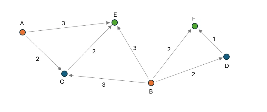
The image above illustrates a minimum cost flow optimization problem with six nodes and eight edges. Nodes A and B serve as sources, each with a supply of 50 units, while nodes E and F act as sinks, each with a demand of 40 units. Every edge has a maximum capacity of 25 units, with variable costs indicated in the image. The objective of the optimization is to allocate flow on each edge to move the required units from nodes A and B to nodes E and F, respecting the edge capacities at the lowest possible cost.

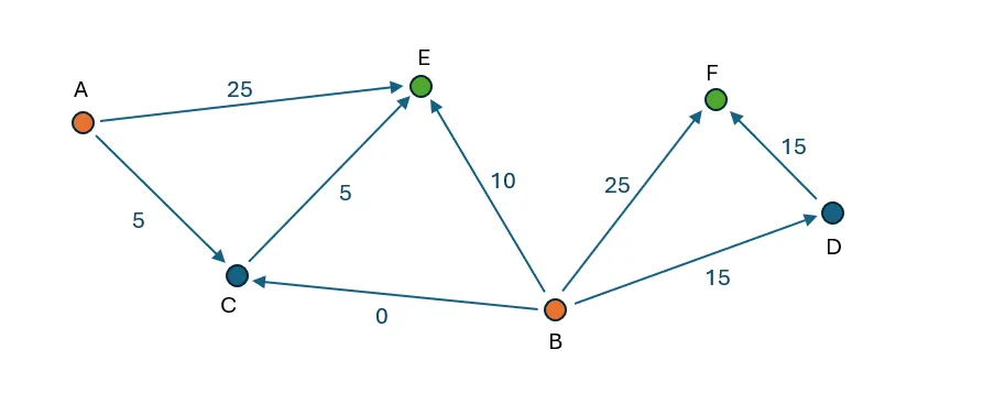
Node F can only receive supply from node B. There are two paths: directly or through node D. The direct path has a cost of 2, while the indirect path via D has a combined cost of 3. Thus, 25 units (the maximum edge capacity) are moved directly from B to F. The remaining 15 units are routed via B -D-F to meet the demand.

Currently, 40 out of 50 units have been transferred from node B, leaving a remaining supply of 10 units that can be moved to node E. The available pathways for supplying node E include: A-E and B-E with a cost of 3, A-C-E with a cost of 4, and B-C-E with a cost of 5. Consequently, 25 units are transported from A-E (limited by the edge capacity) and 10 units from B-E (limited by the remaining supply at node B). To meet the demand of 40 units at node E, an additional 5 units are moved via A-C-E, resulting in no flow being allocated to the B-C pathway.

Mathematical formulation

I introduce two mathematical formulations of minimum cost flow optimization:

1. LP (linear program) with continuous variables only

2. MILP (mixed integer linear program) with continuous and discrete variables

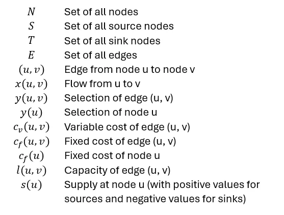
I am using following definitions:

Definitions

LP formulation

This formulation only contains decision variables that are continuous, meaning they can have any value as long as all constraints are fulfilled. Decision variables are in this case the flow variables x(u, v) of all edges.

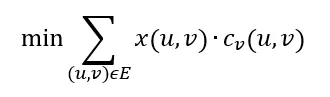
The objective function describes how the costs that are supposed to be minimized are calculated. In this case it is defined as the flow multiplied with the variable cost summed up over all edges:

Constraints are conditions that must be satisfied for the solution to be valid, ensuring that the flow does not exceed capacity limitations.

First, all flows must be non-negative and not exceed to edge capacities:

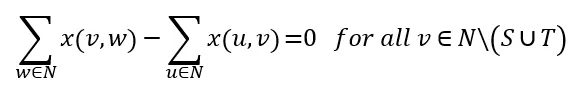
Flow conservation constraints ensure that the same amount of flow that goes into a node has to come out of the node. These constraints are applied to all nodes that are neither sources nor sinks:

For source and sink nodes the difference of out flow and in flow is smaller or equal the supply of the node:

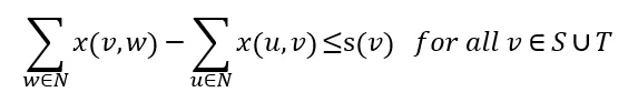
If v is a source the difference of outflow minus inflow must not exceed the supply s(v). In case v is a sink node we do not allow that more than -s(v) can flow into the node than out of the node (for sinks s(v) is negative).

MILP

Additionally, to the continuous variables of the LP formulation, the MILP formulation also contains discreate variables that can only have specific values. Discrete variables allow to restrict the number of used nodes or edges to certain values. It can also be used to introduce fixed costs for using nodes or edges. In this article I show how to add fixed costs. It is important to note that adding discrete decision variables makes it much more difficult to find an optimal solution, hence this formulation should only be used if a LP formulation is not possible.

The objective function is defined as:

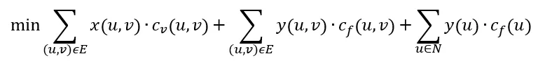
With three terms: variable cost of all edges, fixed cost of all edges, and fixed cost of all nodes.

The maximum flow that can be allocated to an edge depends on the edge’s capacity, the edge selection variable, and the origin node selection variable:

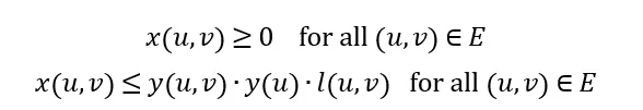
This equation ensures that flow can only be assigned to edges if the edge selection variable and the origin node selection variable are 1.

The flow conservation constraints are equivalent to the LP problem.

Implementation

In this section I explain how to implement a MILP optimization in Python. You can find the code in this repo.

Libraries

To build the flow network, I used NetworkX which is an excellent library (https://networkx.org/) for working with graphs. There are many interesting articles that demonstrate how powerful and easy to use NetworkX is to work with graphs, i.a. customizing NetworkX GraphsNetworkX: Code Demo for Manipulating SubgraphsSocial Network Analysis with NetworkX: A Gentle Introduction.

One important aspect when building an optimization is to make sure that the input is correctly defined. Even one small error can make the problem infeasible or can lead to an unexpected solution. To avoid this, I used Pydantic to validate the user input and raise any issues at the earliest possible stage. This article gives an easy to understand introduction to Pydantic.

To transform the defined network into a mathematical optimization problem I used PuLP. Which allows to define all variables and constraint in an intuitive way. This library also has the advantage that it can use many different solvers in a simple pug-and-play fashion. This article provides good introduction to this library.

Defining nodes and edges

The code below shows how nodes are defined:

from pydantic import BaseModel, model_validator
from typing import Optional

# node and edge definitions
class Node(BaseModel, frozen=True):
    """
    class of network node with attributes:
    name: str - name of node
    demand: float - demand of node (if node is sink)
    supply: float - supply of node (if node is source)
    capacity: float - maximum flow out of node
    type: str - type of node
    x: float - x-coordinate of node
    y: float - y-coordinate of node
    fixed_cost: float - cost of selecting node
    """
    name: str
    demand: Optional[float] = 0.0
    supply: Optional[float] = 0.0
    capacity: Optional[float] = float('inf')
    type: Optional[str] = None
    x: Optional[float] = 0.0
    y: Optional[float] = 0.0
    fixed_cost: Optional[float] = 0.0

    @model_validator(mode='after')
    def validate(self):
        """
        validate if node definition are correct
        """
        # check that demand is non-negative
        if self.demand < 0 or self.demand == float('inf'): raise ValueError('demand must be non-negative and finite')
        # check that supply is non-negative
        if self.supply < 0: raise ValueError('supply must be non-negative')
        # check that capacity is non-negative
        if self.capacity < 0: raise ValueError('capacity must be non-negative')
        # check that fixed_cost is non-negative
        if self.fixed_cost < 0: raise ValueError('fixed_cost must be non-negative')
        return self

Nodes are defined through the Node class which is inherited from Pydantic’s BaseModel. This enables an automatic validation that ensures that all properties are defined with the correct datatype whenever a new object is created. In this case only the name is a required input, all other properties are optional, if they are not provided the specified default value is assigned to them. By setting the “frozen” parameter to True I made all properties immutable, meaning they cannot be changed after the object has been initialized.

The validate method is executed after the object has been initialized and applies more checks to ensure the provided values are as expected. Specifically it checks that demand, supply, capacity, variable cost and fixed cost are not negative. Furthermore, it also does not allow infinite demand as this would lead to an infeasible optimization problem.

These checks look trivial, however their main benefit is that they will trigger an error at the earliest possible stage when an input is incorrect. Thus, they prevent creating a optimization model that is incorrect. Exploring why a model cannot be solved would be much more time consuming as there are many factors that would need to be analyzed, while such “trivial” input error may not be the first aspect to investigate.

Edges are implemented as follows:

class Edge(BaseModel, frozen=True):
"""
class of edge between two nodes with attributes:
origin: 'Node' - origin node of edge
destination: 'Node' - destination node of edge
capacity: float - maximum flow through edge
variable_cost: float - cost per unit flow through edge
fixed_cost: float - cost of selecting edge
"""
origin: Node
destination: Node
capacity: Optional[float] = float('inf')
variable_cost: Optional[float] = 0.0
fixed_cost: Optional[float] = 0.0

@model_validator(mode='after')
def validate(self):
"""
validate of edge definition is correct
"""
# check that node names are different
if self.origin.name == self.destination.name: raise ValueError('origin and destination names must be different')
# check that capacity is non-negative
if self.capacity < 0: raise ValueError('capacity must be non-negative')
# check that variable_cost is non-negative
if self.variable_cost < 0: raise ValueError('variable_cost must be non-negative')
# check that fixed_cost is non-negative
if self.fixed_cost < 0: raise ValueError('fixed_cost must be non-negative')
return self

The required inputs are an origin node and a destination node object. Additionally, capacity, variable cost and fixed cost can be provided. The default value for capacity is infinity which means if no capacity value is provided it is assumed the edge does not have a capacity limitation. The validation ensures that the provided values are non-negative and that origin node name and the destination node name are different.

Initialization of flowgraph object

To define the flowgraph and optimize the flow I created a new class called FlowGraph that is inherited from NetworkX’s DiGraph class. By doing this I can add my own methods that are specific to the flow optimization and at the same time use all methods DiGraph provides:

from networkx import DiGraph
from pulp import LpProblem, LpVariable, LpMinimize, LpStatus

class FlowGraph(DiGraph):
    """
    class to define and solve minimum cost flow problems
    """
    def __init__(self, nodes=[], edges=[]):
        """
        initialize FlowGraph object
        :param nodes: list of nodes
        :param edges: list of edges
        """
        # initialialize digraph
        super().__init__(None)

        # add nodes and edges
        for node in nodes: self.add_node(node)
        for edge in edges: self.add_edge(edge)


    def add_node(self, node):
        """
        add node to graph
        :param node: Node object
        """
        # check if node is a Node object
        if not isinstance(node, Node): raise ValueError('node must be a Node object')
        # add node to graph
        super().add_node(node.name, demand=node.demand, supply=node.supply, capacity=node.capacity, type=node.type, 
                         fixed_cost=node.fixed_cost, x=node.x, y=node.y)
        
    
    def add_edge(self, edge):    
        """
        add edge to graph
        @param edge: Edge object
        """   
        # check if edge is an Edge object
        if not isinstance(edge, Edge): raise ValueError('edge must be an Edge object')
        # check if nodes exist
        if not edge.origin.name in super().nodes: self.add_node(edge.origin)
        if not edge.destination.name in super().nodes: self.add_node(edge.destination)

        # add edge to graph
        super().add_edge(edge.origin.name, edge.destination.name, capacity=edge.capacity, 
                         variable_cost=edge.variable_cost, fixed_cost=edge.fixed_cost)

FlowGraph is initialized by providing a list of nodes and edges. The first step is to initialize the parent class as an empty graph. Next, nodes and edges are added via the methods add_node and add_edge. These methods first check if the provided element is a Node or Edge object. If this is not the case an error will be raised. This ensures that all elements added to the graph have passed the validation of the previous section. Next, the values of these objects are added to the Digraph object. Note that the Digraph class also uses add_node and add_edge methods to do so. By using the same method name I am overwriting these methods to ensure that whenever a new element is added to the graph it must be added through the FlowGraph methods which validate the object type. Thus, it is not possible to build a graph with any element that has not passed the validation tests.

Initializing the optimization problem

The method below converts the network into an optimization model, solves it, and retrieves the optimized values.

  def min_cost_flow(self, verbose=True):
        """
        run minimum cost flow optimization
        @param verbose: bool - print optimization status (default: True)
        @return: status of optimization
        """
        self.verbose = verbose

        # get maximum flow
        self.max_flow = sum(node['demand'] for _, node in super().nodes.data() if node['demand'] > 0)

        start_time = time.time()
        # create LP problem
        self.prob = LpProblem("FlowGraph.min_cost_flow", LpMinimize)
        # assign decision variables
        self._assign_decision_variables()
        # assign objective function
        self._assign_objective_function()
        # assign constraints
        self._assign_constraints()
        if self.verbose: print(f"Model creation time: {time.time() - start_time:.2f} s")

        start_time = time.time()
        # solve LP problem
        self.prob.solve()
        solve_time = time.time() - start_time

        # get status
        status = LpStatus[self.prob.status]

        if verbose:
            # print optimization status
            if status == 'Optimal':
                # get objective value
                objective = self.prob.objective.value()
                print(f"Optimal solution found: {objective:.2f} in {solve_time:.2f} s")
            else:
                print(f"Optimization status: {status} in {solve_time:.2f} s")
        
        # assign variable values
        self._assign_variable_values(status=='Optimal')

        return status

Pulp’s LpProblem is initialized, the constant LpMinimize defines it as a minimization problem — meaning it is supposed to minimize the value of the objective function. In the following lines all decision variables are initialized, the objective function as well as all constraints are defined. These methods will be explained in the following sections.

Next, the problem is solved, in this step the optimal value of all decision variables is determined. Following the status of the optimization is retrieved. When the status is “Optimal” an optimal solution could be found other statuses are “Infeasible” (it is not possible to fulfill all constraints), “Unbounded” (the objective function can have an arbitrary low values), and “Undefined” meaning the problem definition is not complete. In case no optimal solution was found the problem definition needs to be reviewed.

Finally, the optimized values of all variables are retrieved and assigned to the respective nodes and edges.

Defining decision variables

All decision variables are initialized in the method below:

   def _assign_variable_values(self, opt_found):
        """
        assign decision variable values if optimal solution found, otherwise set to None
        @param opt_found: bool - if optimal solution was found
        """
        # assign edge values        
        for _, _, edge in super().edges.data():
            # initialize values
            edge['flow'] = None
            edge['selected'] = None
            # check if optimal solution found
            if opt_found and edge['flow_var'] is not None:                    
                edge['flow'] = edge['flow_var'].varValue                    

                if edge['selection_var'] is not None: 
                    edge['selected'] = edge['selection_var'].varValue

        # assign node values
        for _, node in super().nodes.data():
            # initialize values
            node['selected'] = None
            if opt_found:                
                # check if node has selection variable
                if node['selection_var'] is not None: 
                    node['selected'] = node['selection_var'].varValue

First it iterates through all edges and assigns continuous decision variables if the edge capacity is greater than 0. Furthermore, if fixed costs of the edge are greater than 0 a binary decision variable is defined as well. Next, it iterates through all nodes and assigns binary decision variables to nodes with fixed costs. The total number of continuous and binary decision variables is counted and printed at the end of the method.

Defining objective

After all decision variables have been initialized the objective function can be defined:

    def _assign_objective_function(self):
        """
        define objective function
        """
        objective = 0
 
        # add edge costs
        for _, _, edge in super().edges.data():
            if edge['selection_var'] is not None: objective += edge['selection_var'] * edge['fixed_cost']
            if edge['flow_var'] is not None: objective += edge['flow_var'] * edge['variable_cost']
        
        # add node costs
        for _, node in super().nodes.data():
            # add node selection costs
            if node['selection_var'] is not None: objective += node['selection_var'] * node['fixed_cost']

        self.prob += objective, 'Objective',

The objective is initialized as 0. Then for each edge fixed costs are added if the edge has a selection variable, and variable costs are added if the edge has a flow variable. For all nodes with selection variables fixed costs are added to the objective as well. At the end of the method the objective is added to the LP object.

Defining constraints

All constraints are defined in the method below:

  def _assign_constraints(self):
        """
        define constraints
        """
        # count of contraints
        constr_count = 0
        # add capacity constraints for edges with fixed costs
        for origin_name, destination_name, edge in super().edges.data():
            # get capacity
            capacity = edge['capacity'] if edge['capacity'] < float('inf') else self.max_flow
            rhs = capacity
            if edge['selection_var'] is not None: rhs *= edge['selection_var']
            self.prob += edge['flow_var'] <= rhs, f"capacity_{origin_name}-{destination_name}",
            constr_count += 1
            
            # get origin node
            origin_node = super().nodes[origin_name]
            # check if origin node has a selection variable
            if origin_node['selection_var'] is not None:
                rhs = capacity * origin_node['selection_var'] 
                self.prob += (edge['flow_var'] <= rhs, f"node_selection_{origin_name}-{destination_name}",)
                constr_count += 1

        total_demand = total_supply = 0
        # add flow conservation constraints
        for node_name, node in super().nodes.data():
            # aggregate in and out flows
            in_flow = 0
            for _, _, edge in super().in_edges(node_name, data=True):
                if edge['flow_var'] is not None: in_flow += edge['flow_var']
            
            out_flow = 0
            for _, _, edge in super().out_edges(node_name, data=True):
                if edge['flow_var'] is not None: out_flow += edge['flow_var']

            # add node capacity contraint
            if node['capacity'] < float('inf'):
                self.prob += out_flow = demand - supply
                rhs = node['demand'] - node['supply']
                self.prob += in_flow - out_flow >= rhs, f"flow_balance_{node_name}",
            constr_count += 1

            # update total demand and supply
            total_demand += node['demand']
            total_supply += node['supply']

        if self.verbose:
            print(f"Constraints: {constr_count}")
            print(f"Total supply: {total_supply}, Total demand: {total_demand}")

First, capacity constraints are defined for each edge. If the edge has a selection variable the capacity is multiplied with this variable. In case there is no capacity limitation (capacity is set to infinity) but there is a selection variable, the selection variable is multiplied with the maximum flow that has been calculated by aggregating the demand of all nodes. An additional constraint is added in case the edge’s origin node has a selection variable. This constraint means that flow can only come out of this node if the selection variable is set to 1.

Following, the flow conservation constraints for all nodes are defined. To do so the total in and outflow of the node is calculated. Getting all in and outgoing edges can easily be done by using the in_edges and out_edges methods of the DiGraph class. If the node has a capacity limitation the maximum outflow will be constraint by that value. For the flow conservation it is necessary to check if the node is either a source or sink node or a transshipment node (demand equals supply). In the first case the difference between inflow and outflow must be greater or equal the difference between demand and supply while in the latter case in and outflow must be equal.

The total number of constraints is counted and printed at the end of the method.

Retrieving optimized values

After running the optimization, the optimized variable values can be retrieved with the following method:

    def _assign_variable_values(self, opt_found):
        """
        assign decision variable values if optimal solution found, otherwise set to None
        @param opt_found: bool - if optimal solution was found
        """
        # assign edge values        
        for _, _, edge in super().edges.data():
            # initialize values
            edge['flow'] = None
            edge['selected'] = None
            # check if optimal solution found
            if opt_found and edge['flow_var'] is not None:                    
                edge['flow'] = edge['flow_var'].varValue                    

                if edge['selection_var'] is not None: 
                    edge['selected'] = edge['selection_var'].varValue

        # assign node values
        for _, node in super().nodes.data():
            # initialize values
            node['selected'] = None
            if opt_found:                
                # check if node has selection variable
                if node['selection_var'] is not None: 
                    node['selected'] = node['selection_var'].varValue 

This method iterates through all edges and nodes, checks if decision variables have been assigned and adds the decision variable value via varValue to the respective edge or node.

Demo

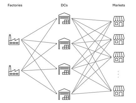
To demonstrate how to apply the flow optimization I created a supply chain network consisting of 2 factories, 4 distribution centers (DC), and 15 markets. All goods produced by the factories have to flow through one distribution center until they can be delivered to the markets.

Supply chain problem

Node properties were defined:

Node definitions

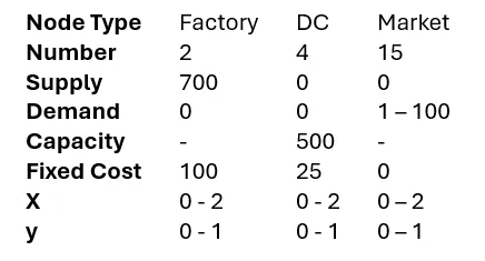
Ranges mean that uniformly distributed random numbers were generated to assign these properties. Since Factories and DCs have fixed costs the optimization also needs to decide which of these entities should be selected.

Edges are generated between all Factories and DCs, as well as all DCs and Markets. The variable cost of edges is calculated as the Euclidian distance between origin and destination node. Capacities of edges from Factories to DCs are set to 350 while from DCs to Markets are set to 100.

The code below shows how the network is defined and how the optimization is run:

# Define nodes
factories = [Node(name=f'Factory {i}', supply=700, type='Factory', fixed_cost=100, x=random.uniform(0, 2),
                  y=random.uniform(0, 1)) for i in range(2)]
dcs = [Node(name=f'DC {i}', fixed_cost=25, capacity=500, type='DC', x=random.uniform(0, 2), 
            y=random.uniform(0, 1)) for i in range(4)]
markets = [Node(name=f'Market {i}', demand=random.randint(1, 100), type='Market', x=random.uniform(0, 2), 
                y=random.uniform(0, 1)) for i in range(15)]

# Define edges
edges = []
# Factories to DCs
for factory in factories:
    for dc in dcs:
        distance = ((factory.x - dc.x)**2 + (factory.y - dc.y)**2)**0.5
        edges.append(Edge(origin=factory, destination=dc, capacity=350, variable_cost=distance))

# DCs to Markets
for dc in dcs:
    for market in markets:
        distance = ((dc.x - market.x)**2 + (dc.y - market.y)**2)**0.5
        edges.append(Edge(origin=dc, destination=market, capacity=100, variable_cost=distance))

# Create FlowGraph
G = FlowGraph(edges=edges)

G.min_cost_flow()

The output of flow optimization is as follows:

Variable types: 68 continuous, 6 binary
Constraints: 161
Total supply: 1400.0, Total demand: 909.0
Model creation time: 0.00 s
Optimal solution found: 1334.88 in 0.23 s

The problem consists of 68 continuous variables which are the edges’ flow variables and 6 binary decision variables which are the selection variables of the Factories and DCs. There are 161 constraints in total which consist of edge and node capacity constraints, node selection constraints (edges can only have flow if the origin node is selected), and flow conservation constraints. The next line shows that the total supply is 1400 which is higher than the total demand of 909 (if the demand was higher than the supply the problem would be infeasible). Since this is a small optimization problem, the time to define the optimization model was less than 0.01 seconds. The last line shows that an optimal solution with an objective value of 1335 could be found in 0.23 seconds.

Additionally, to the code I described in this post I also added two methods that visualize the optimized solution. The code of these methods can also be found in the repo.

Flow graph

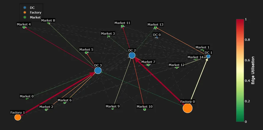
All nodes are located by their respective x and y coordinates. The node and edge size is relative to the total volume that is flowing through. The edge color refers to its utilization (flow over capacity). Dashed lines show edges without flow allocation.

In the optimal solution both Factories were selected which is inevitable as the maximum supply of one Factory is 700 and the total demand is 909. However, only 3 of the 4 DCs are used (DC 0 has not been selected).

In general the plot shows the Factories are supplying the nearest DCs and DCs the nearest Markets. However, there are a few exceptions to this observation: Factory 0 also supplies DC 3 although Factory 1 is nearer. This is due to the capacity constraints of the edges which only allow to move at most 350 units per edge. However, the closest Markets to DC 3 have a slightly higher demand, hence Factory 0 is moving additional units to DC 3 to meet that demand. Although Market 9 is closest to DC 3 it is supplied by DC 2. This is because DC 3 would require an additional supply from Factory 0 to supply this market and since the total distance from Factory 0 over DC 3 is longer than the distance from Factory 0 through DC 2, Market 9 is supplied via the latter route.

Another way to visualize the results is via a Sankey diagram which focuses on visualizing the flows of the edges:

Sankey flow diagram

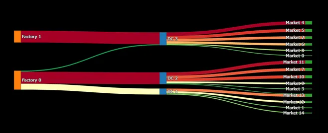
The colors represent the edges’ utilizations with lowest utilizations in green changing to yellow and red for the highest utilizations. This diagram shows very well how much flow goes through each node and edge. It highlights the flow from Factory 0 to DC 3 and also that Market 13 is supplied by DC 2 and DC 1.

Summary

Minimum cost flow optimizations can be a very helpful tool in many domains like logistics, transportation, telecommunication, energy sector and many more. To apply this optimization it is important to translate a physical system into a mathematical graph consisting of nodes and edges. This should be done in a way to have as few discrete (e.g. binary) decision variables as necessary as those make it significantly more difficult to find an optimal solution. By combining Python’s NetworkX, Pulp and Pydantic libraries I built an flow optimization class that is intuitive to initialize and at the same time follows a generalized formulation which allows to apply it in many different use cases. Graph and flow diagrams are very helpful to understand the solution found by the optimizer.

If not otherwise stated all images were created by the author.

Shape
Shape
Stay Ahead

Explore More Insights

Stay ahead with more perspectives on cutting-edge power, infrastructure, energy,  bitcoin and AI solutions. Explore these articles to uncover strategies and insights shaping the future of industries.

Shape

Cloudflare wants to rebuild the network for the age of AI agents

Setup: Cano explained that users go from zero to a working private network in under five minutes through a dashboard wizard, with no networking expertise required.  Bidirectional: This means every device and server gets a private IP and can reach every other device and server, not just client-to-server, but server-to-server,

Read More »

AI fuels wireless talent shortage

Among organizations struggling to hire, 85% expect wireless security failures to increase over the next two years, compared to 59% of those without hiring difficulty. According to Cisco, “85% of organizations experienced a wireless security incident in the past year, and 54% report that threats are increasing in frequency and

Read More »

Energy Department Awards New Contracts from Strategic Petroleum Reserve, Advancing Emergency Exchange

WASHINGTON—The U.S. Department of Energy’s (DOE) Hydrocarbons and Geothermal Energy Office (HGEO) today announced awards of contracts to exchange 26 million barrels of crude oil from the Strategic Petroleum Reserve (SPR) at the West Hackberry site, marking the next phase of DOE’s execution of the United States’ 172-million-barrel contribution to the International Energy Agency’s collective action to stabilize global oil supply. These awards follow DOE’s recent Request for Proposal (RFP) for this portion of the emergency exchange, with deliveries beginning immediately as the Department continues to move quickly to address short-term supply disruptions and strengthen energy security for the United States. “Through this emergency exchange, the Department is taking swift action to support near‑term supply needs while strengthening the Strategic Petroleum Reserve for the long term,” said Kyle Haustveit, Assistant Secretary of the Hydrocarbons and Geothermal Energy Office. “By returning additional premium barrels at no cost to taxpayers, this exchange reinforces market reliability today and delivers meaningful value to the American people when those barrels are returned.” Under these awards, DOE will move forward with an exchange of 26 million barrels of crude oil, which will be returned with additional premium barrels by next year—supporting energy security and delivering value for the American people at no cost to taxpayers. This action builds on earlier exchange actions, which have already awarded approximately 55 million barrels from the Bayou Choctaw, Bryan Mound, and West Hackberry sites, demonstrating the reserve’s ability to deliver crude efficiently under emergency conditions. To date, more than 10 million barrels have already been delivered to market. The exchange also allows participating companies to take advantage of the President’s limited Jones Act waiver, helping accelerate critical near-term oil flows into the market. Companies can begin scheduling deliveries immediately. DOE will continue to evaluate market conditions and operational capacity as it advances

Read More »

Apply Now: 2026 Waste to Energy and Materials Technical Assistance for State, Local, and Tribal Governments

The U.S. Department of Energy’s Alternative Fuels and Feedstocks Office (AFFO), formerly known as the Bioenergy Technologies Office, and the National Laboratory of the Rockies (NLR) are launching the 2026 Waste to Energy and Materials Technical Assistance Program for state, local, and Tribal governments. The scope of this year’s program has been expanded to include additional municipal solid waste materials such as electronics, industrial wastewater, and other byproducts.  U.S. waste streams present significant logistical and economic challenges for states, counties, municipalities, and Tribal governments. However, waste is also a resource that can be used as an unconventional additional source of energy, advanced materials, and critical minerals. This program provides no-cost technical assistance to states, counties, municipalities, and Tribal governments with the most relevant data to guide decision-making—providing local solutions to the various aspects of waste management, taking into consideration current handling practices, costs, and infrastructure. It is designed to help officials evaluate the most sensible end uses for their waste, whether repurposing it for on-site heat and power, upgrading it into transportation fuels, or using it for material and mineral recovery. Program technical assistance includes: Waste resource information Infrastructure considerations Techno-economic comparison of energy, material, and mineral recovery options Evaluation and sharing of case studies (to the extent possible) from similar communities/projects The 2026 Waste to Energy and Materials Technical Assistance application portal is now open and applications will be accepted through May 30, 2026. For information on applicant eligibility and how to apply, please visit NLR’s technical assistance webpage. Timeline for Technical Assistance Opportunity Date Action April 15, 2026 Application Portal Opens May 30, 2026 Application Portal Closes  July – August 2026 Selections Made and Recipients Informed  Learn more about AFFO-supported waste to energy and materials technical assistance. If you have further questions, please see frequently asked questions or contact the Waste to

Read More »

Energy Deputy Secretary Danly Commends FERC Action on Large Load Interconnection Reform

WASHINGTON—U.S. Deputy Secretary of Energy James P. Danly issued the following statement after the Federal Energy Regulatory Commission (FERC or Commission) announced it will take action by June 2026 on the large load interconnection proceeding initiated at the direction of U.S. Secretary of Energy Chris Wright: “FERC’s announcement today demonstrates Chairman Swett’s commitment to implement Secretary Wright’s directive that the Commission ensure the timely and orderly integration of large electric loads that deliver on President Trump’s goal of American energy dominance. “I expect that the Commission will act quickly and decisively to improve interconnection processes, support the co-location of load and generation, and accelerate the addition of new generation to ensure that supply is built alongside demand—delivering affordable, reliable, and secure energy for all Americans. “Having served at FERC as commissioner and chairman, I understand FERC’s role in ensuring the reliability of the nation’s bulk power system, and I commend Chairman Swett for focusing on affordability and reliability.”                                                                                               ###  

Read More »

Petrobras discovers hydrocarbons in Campos basin presalt offshore Brazil

@import url(‘https://fonts.googleapis.com/css2?family=Inter:[email protected]&display=swap’); .ebm-page__main h1, .ebm-page__main h2, .ebm-page__main h3, .ebm-page__main h4, .ebm-page__main h5, .ebm-page__main h6 { font-family: Inter; } body { line-height: 150%; letter-spacing: 0.025em; } button, .ebm-button-wrapper { font-family: Inter; } .label-style { text-transform: uppercase; color: var(–color-grey); font-weight: 600; font-size: 0.75rem; } .caption-style { font-size: 0.75rem; opacity: .6; } #onetrust-pc-sdk [id*=btn-handler], #onetrust-pc-sdk [class*=btn-handler] { background-color: #c19a06 !important; border-color: #c19a06 !important; } #onetrust-policy a, #onetrust-pc-sdk a, #ot-pc-content a { color: #c19a06 !important; } #onetrust-consent-sdk #onetrust-pc-sdk .ot-active-menu { border-color: #c19a06 !important; } #onetrust-consent-sdk #onetrust-accept-btn-handler, #onetrust-banner-sdk #onetrust-reject-all-handler, #onetrust-consent-sdk #onetrust-pc-btn-handler.cookie-setting-link { background-color: #c19a06 !important; border-color: #c19a06 !important; } #onetrust-consent-sdk .onetrust-pc-btn-handler { color: #c19a06 !important; border-color: #c19a06 !important; } Petrobras has discovered presence in the Campos basin presalt offshore Brazil during exploration in sector SC-AP4, block CM-477. Samples taken from the well, 1-BRSA-1404DC-RJS, will be sent for laboratory analysis with the aim of characterizing the conditions of the reservoirs and fluids found to enable continued evaluation of the area’s potential, the company said in a release Apr. 13. The discovery well was drilled 201 km off the coast of the state of Rio de Janeiro in water depth of 2,984 m. The hydrocarbon-bearing interval was confirmed through electrical profiles, gas evidence, and fluid sampling. Petrobras is the operator of block CM-477 with 70% interest. bp plc holds the remaining 30%.

Read More »

bp to operate blocks offshore Namibia through acquisition

@import url(‘https://fonts.googleapis.com/css2?family=Inter:[email protected]&display=swap’); .ebm-page__main h1, .ebm-page__main h2, .ebm-page__main h3, .ebm-page__main h4, .ebm-page__main h5, .ebm-page__main h6 { font-family: Inter; } body { line-height: 150%; letter-spacing: 0.025em; } button, .ebm-button-wrapper { font-family: Inter; } .label-style { text-transform: uppercase; color: var(–color-grey); font-weight: 600; font-size: 0.75rem; } .caption-style { font-size: 0.75rem; opacity: .6; } #onetrust-pc-sdk [id*=btn-handler], #onetrust-pc-sdk [class*=btn-handler] { background-color: #c19a06 !important; border-color: #c19a06 !important; } #onetrust-policy a, #onetrust-pc-sdk a, #ot-pc-content a { color: #c19a06 !important; } #onetrust-consent-sdk #onetrust-pc-sdk .ot-active-menu { border-color: #c19a06 !important; } #onetrust-consent-sdk #onetrust-accept-btn-handler, #onetrust-banner-sdk #onetrust-reject-all-handler, #onetrust-consent-sdk #onetrust-pc-btn-handler.cookie-setting-link { background-color: #c19a06 !important; border-color: #c19a06 !important; } #onetrust-consent-sdk .onetrust-pc-btn-handler { color: #c19a06 !important; border-color: #c19a06 !important; } Map from bp plc <!–> –> bp plc aims to become operator of three exploration blocks offshore Namibia through acquisition of a 60% interest from Eco Atlantic Oil & Gas. Subject to Namibian government and joint venture partner approvals, bp will operate blocks PEL97, PEL99, and PEL100 in Walvis basin.   In a release Apr. 13, bp said entering the blocks builds on its recent exploration successes in Namibia through Azule Energy, a 50-50 joint venture between bp and Eni. Eco Atlantic will remain a partner, along with Namibia’s national oil company NAMCOR, following the deal’s closing, which is subject to closing conditions.

Read More »

ConocoPhillips sends team to Venezuela to evaluate oil, gas opportunities

ConocoPhillips sent a team to Venezuela to evaluate oil and gas opportunities, the company confirmed to Oil & Gas Journal Apr. 13. In an email to OGJ, a company spokesperson said “ConocoPhillips can confirm that we sent a small evaluation team to Venezuela during the week of Apr. 6 to better understand the potential for in-country oil and gas opportunities.” Asked what clarity the company seeks, the spokesperson said the team “will evaluate Venezuela against other international opportunities as part of our disciplined investment framework.” The operator left Venezuela in 2007 after then-President Hugo Chavez’s government reverted privately run oil fields to state control. ConocoPhillips, along with ExxonMobil, refused the government’s terms and took claims to the World Bank’s International Centre for the Settlement of Investment Disputes (ICSID). ConocoPhillips is owed about $12 billion following two judgements, an amount still sought by the company, which, prior to the expropriation of its interests, held a 50.1% interest in Petrozuata, a 40% interest in Hamaca, and a 32.5% interest in Corocoro heavy oil projects in Venezuela. In January, following the removal of Venezuela’s leader Nicolas Maduro, US President Donald Trump urged oil and gas companies to spend billions to rebuild Venezuela’s energy sector. ExxonMobil, which also exited the country in 2007, ​sent a technical team to Venezuela in March to ⁠evaluate the infrastructure and investment opportunities. In a discussion at CERAWeek by S&P Global in Houston in March, ConocoPhillips’ chief executive officer, Ryan Lance, said Venezuela needs to “completely rewire” ​its fiscal system to attract new ‌investment. The South American country holds a large cache of proven oil reserves, but has faced decades of production challenges due to mismanagement, underinvestment, and sanctions.

Read More »

Data centers are costing local governments billions

Tax benefits for hyperscalers and other data center operators are costing local administrations billions of dollars. In the US, three states are already giving away more than $1 billion in potential tax revenue, while 14 are failing to declare how much data center subsidies are costing taxpayers, according to Good Jobs First. The campaign group said the failure to declare the tax subsidies goes against US Generally Accepted Accounting Principles (GAAP) and that they should, since 2017, be declared as lost revenue. “Tax-abatement laws written long ago for much smaller data centers, predating massive artificial intelligence (AI) facilities, are now unexpectedly costing governments billions of dollars in lost tax revenue,” Good Jobs First said. “Three states, Georgia, Virginia, and Texas, already lose $1 billion or more per year,” it reported in its new study, “Data Center Tax Abatements: Why States and Localities Must Disclose These Soaring Revenue Losses.”

Read More »

Equinix offering targets automated AI-centric network operations

Another component, Fabric Application Connect, functions as a private, dedicated connectivity marketplace for AI services. It lets enterprises access inference, training, storage, and security providers over private connections, bypassing the public Internet and limiting data exposure during AI development and deployment. Operational visibility is provided through Fabric Insights, an AI-powered monitoring layer that analyzes real-time network telemetry to detect anomalies and predict potential issues before they impact workloads. Fabric Insights integrates with security information and event management (SIEM) platforms such as Splunk and Datadog and feeds data directly into Fabric Super-Agent to support automated remediation. Fabric Intelligence operates on top of Equinix’s global infrastructure footprint, which includes hundreds of data centers across dozens of metropolitan markets. The platform is positioned as part of Equinix Fabric, a connectivity portfolio used by thousands of customers worldwide to link cloud providers, enterprises, and network services. Fabric Intelligence is available now to preview.

Read More »

Blue Owl Builds a Capital Platform for the Hyperscale AI Era

Capital as a Service: The Hyperscaler Shift This is not just another project financing. It points to a model in which hyperscalers can externalize a significant portion of the capital required for AI campuses while retaining operational control. Under the Hyperion structure, Meta provides construction and property management, while Blue Owl supplies capital at scale alongside infrastructure expertise. Reuters described the transaction as Meta’s largest private capital deal to date, with the campus projected to exceed 2 gigawatts of capacity. For Blue Owl, it marks a shift in role: from backing developers serving hyperscalers to working directly with a hyperscaler to structure ownership more efficiently at scale. Hyperion also helps explain why this model is gaining traction. Hyperscalers are now deploying capital at a pace that makes flexibility a strategic priority. Structures like the Meta–Blue Owl JV allow them to continue expanding infrastructure without fully absorbing the balance-sheet impact of each new campus. Analyst commentary cited by Reuters suggested the arrangement could help Meta mitigate risk and avoid concentrating too much capital in land, buildings, and long-lived infrastructure, preserving capacity for additional facilities and ongoing AI investment. That is the service Blue Owl is effectively providing. Not just capital, but balance-sheet flexibility at a time when AI infrastructure demand is stretching even the largest technology companies. With major tech firms projected to spend hundreds of billions annually on AI infrastructure, that capability is becoming central to how the next generation of campuses gets built. The Capital Baseline Resets In early 2026, hyperscalers effectively reset the capital baseline for the sector. Alphabet projected $175 billion to $185 billion in annual capex, citing continued constraints across servers, data centers, and networking. Amazon pointed to roughly $200 billion, up from $131 billion the prior year, while noting persistent demand pressure in AWS. Meta

Read More »

OpenAI pulls out of a second Stargate data center deal

“OpenAI is embattled on several fronts. Anthropic has been doing very well in the enterprise, and OpenAI’s cash burn might be a problem if it wants to go public at an astronomical $800 billion+ valuation. This is especially true with higher energy prices due to geopolitics, and the public and regulators increasingly skeptical of AI companies, especially outside of the United States,” Roberts said. “I see these moves as OpenAI tightening its belt a bit and being more deliberate about spending as it moves past the interesting tech demo stage of its existence and is expected to provide a real return for investors.” He added, “I expect it’s a symptom of a broader problem, which is that OpenAI has thrown some good money after bad in bets that didn’t work out, like the Sora platform it just shut down, and it’s under increasing pressure to translate its first-mover advantage into real upside for its investors. Spending operational money instead of capital money might give it some flexibility in the short term, and perhaps that’s what this is about.” All in all, he noted, “on a scale of business-ending event to nothingburger, I would put it somewhere in the middle, maybe a little closer to nothingburger.” Acceligence CIO Yuri Goryunov agreed with Roberts, and said, “OpenAI has a problem with commercialization and runaway operating costs, for sure. They are trying to rightsize their commitments and make sure that they deliver on their core products before they run out of money.” Goryunov described OpenAI’s arrangement with Microsoft in Norway as “prudent financial engineering” that allows it to access the data center resources without having to tie up too much capital. “It’s financial discipline. OpenAI [executives] are starting to behave like grownups.” Forrester senior analyst Alvin Nguyen echoed those thoughts. 

Read More »

DCF Tours: SDC Manhattan, 375 Pearl St.

Power: Redundant utility design in a power-constrained market The tour made equally clear that in Manhattan, power is still the central gating factor. The brochure describes SDC Manhattan as offering 18MW of aggregate power delivered to the building, backed by redundant electrical and mechanical systems, backup generators, and Tier III-type concurrent maintainability. The December 2025 press release updated that picture in a more market-facing way, noting that Sabey is one of the only colocation providers in Manhattan with available power, including nearly a megawatt of turnkey power and 7MW of utility power across two powered shell spaces. Bajrushi’s explanation of the electrical topology helped show how Sabey has made that possible. Standing on the third floor, he described a ring bus tying together four Con Edison feeds. Bajrushi said the feeds all originate from the same substation but take different paths into the building, creating redundancy outside the building as well as within it. He added that if one feed fails, the ring bus remains unaffected, and that only one feed is needed to power everything currently in operation. He also noted that Sabey has the ability to add two more feeds in the future if expansion calls for it. That matters in a city where available utility capacity is hard to come by and where many data center conversations end not with square footage but with a megawatt number. Bajrushi also noted that physical space is not the core constraint at 375 Pearl. He said the building still has plenty of room for future buildouts, including open areas that could become additional white space, chiller capacity, or other infrastructure. The bigger question, he suggested, is how and when power and supporting systems get installed. That observation aligns neatly with Sabey’s press release. The company is effectively arguing that SDC

Read More »

Maine to put brakes on big data centers as AI expansion collides with power limits

Mills has pushed for an exemption protecting a proposed $550 million project at the former Androscoggin paper mill in Jay, arguing it would reuse existing infrastructure without straining the grid. Lawmakers rejected that exemption. Mills’ office did not immediately respond to a request for comment. A national wave, an unanswered federal question Maine is one of at least 12 states now weighing moratorium or restraint legislation, alongside more than 300 data center bills filed across 30-plus states in the current session, according to legislative tracking firm MultiState. The shared concern is energy cost. Data centers could consume up to 12% of total US electricity by 2028, according to the US Department of Energy. On March 25, Senator Bernie Sanders and Alexandria Ocasio-Cortez introduced the AI Data Center Moratorium Act in Congress, which would impose a nationwide freeze on all new data center construction until Congress passes AI safety legislation. The Trump administration has pursued a different path from the legislative approach being taken in states. On March 4, Amazon, Google, Meta, Microsoft, OpenAI, Oracle, and xAI signed the White House’s Ratepayer Protection Pledge, a voluntary commitment by hyperscalers to fund their own power generation rather than pass grid costs to ratepayers. The pledge, published in the Federal Register on March 9, carries no penalties for noncompliance or auditing requirements.

Read More »

Microsoft will invest $80B in AI data centers in fiscal 2025

And Microsoft isn’t the only one that is ramping up its investments into AI-enabled data centers. Rival cloud service providers are all investing in either upgrading or opening new data centers to capture a larger chunk of business from developers and users of large language models (LLMs).  In a report published in October 2024, Bloomberg Intelligence estimated that demand for generative AI would push Microsoft, AWS, Google, Oracle, Meta, and Apple would between them devote $200 billion to capex in 2025, up from $110 billion in 2023. Microsoft is one of the biggest spenders, followed closely by Google and AWS, Bloomberg Intelligence said. Its estimate of Microsoft’s capital spending on AI, at $62.4 billion for calendar 2025, is lower than Smith’s claim that the company will invest $80 billion in the fiscal year to June 30, 2025. Both figures, though, are way higher than Microsoft’s 2020 capital expenditure of “just” $17.6 billion. The majority of the increased spending is tied to cloud services and the expansion of AI infrastructure needed to provide compute capacity for OpenAI workloads. Separately, last October Amazon CEO Andy Jassy said his company planned total capex spend of $75 billion in 2024 and even more in 2025, with much of it going to AWS, its cloud computing division.

Read More »

John Deere unveils more autonomous farm machines to address skill labor shortage

Join our daily and weekly newsletters for the latest updates and exclusive content on industry-leading AI coverage. Learn More Self-driving tractors might be the path to self-driving cars. John Deere has revealed a new line of autonomous machines and tech across agriculture, construction and commercial landscaping. The Moline, Illinois-based John Deere has been in business for 187 years, yet it’s been a regular as a non-tech company showing off technology at the big tech trade show in Las Vegas and is back at CES 2025 with more autonomous tractors and other vehicles. This is not something we usually cover, but John Deere has a lot of data that is interesting in the big picture of tech. The message from the company is that there aren’t enough skilled farm laborers to do the work that its customers need. It’s been a challenge for most of the last two decades, said Jahmy Hindman, CTO at John Deere, in a briefing. Much of the tech will come this fall and after that. He noted that the average farmer in the U.S. is over 58 and works 12 to 18 hours a day to grow food for us. And he said the American Farm Bureau Federation estimates there are roughly 2.4 million farm jobs that need to be filled annually; and the agricultural work force continues to shrink. (This is my hint to the anti-immigration crowd). John Deere’s autonomous 9RX Tractor. Farmers can oversee it using an app. While each of these industries experiences their own set of challenges, a commonality across all is skilled labor availability. In construction, about 80% percent of contractors struggle to find skilled labor. And in commercial landscaping, 86% of landscaping business owners can’t find labor to fill open positions, he said. “They have to figure out how to do

Read More »

2025 playbook for enterprise AI success, from agents to evals

Join our daily and weekly newsletters for the latest updates and exclusive content on industry-leading AI coverage. Learn More 2025 is poised to be a pivotal year for enterprise AI. The past year has seen rapid innovation, and this year will see the same. This has made it more critical than ever to revisit your AI strategy to stay competitive and create value for your customers. From scaling AI agents to optimizing costs, here are the five critical areas enterprises should prioritize for their AI strategy this year. 1. Agents: the next generation of automation AI agents are no longer theoretical. In 2025, they’re indispensable tools for enterprises looking to streamline operations and enhance customer interactions. Unlike traditional software, agents powered by large language models (LLMs) can make nuanced decisions, navigate complex multi-step tasks, and integrate seamlessly with tools and APIs. At the start of 2024, agents were not ready for prime time, making frustrating mistakes like hallucinating URLs. They started getting better as frontier large language models themselves improved. “Let me put it this way,” said Sam Witteveen, cofounder of Red Dragon, a company that develops agents for companies, and that recently reviewed the 48 agents it built last year. “Interestingly, the ones that we built at the start of the year, a lot of those worked way better at the end of the year just because the models got better.” Witteveen shared this in the video podcast we filmed to discuss these five big trends in detail. Models are getting better and hallucinating less, and they’re also being trained to do agentic tasks. Another feature that the model providers are researching is a way to use the LLM as a judge, and as models get cheaper (something we’ll cover below), companies can use three or more models to

Read More »

OpenAI’s red teaming innovations define new essentials for security leaders in the AI era

Join our daily and weekly newsletters for the latest updates and exclusive content on industry-leading AI coverage. Learn More OpenAI has taken a more aggressive approach to red teaming than its AI competitors, demonstrating its security teams’ advanced capabilities in two areas: multi-step reinforcement and external red teaming. OpenAI recently released two papers that set a new competitive standard for improving the quality, reliability and safety of AI models in these two techniques and more. The first paper, “OpenAI’s Approach to External Red Teaming for AI Models and Systems,” reports that specialized teams outside the company have proven effective in uncovering vulnerabilities that might otherwise have made it into a released model because in-house testing techniques may have missed them. In the second paper, “Diverse and Effective Red Teaming with Auto-Generated Rewards and Multi-Step Reinforcement Learning,” OpenAI introduces an automated framework that relies on iterative reinforcement learning to generate a broad spectrum of novel, wide-ranging attacks. Going all-in on red teaming pays practical, competitive dividends It’s encouraging to see competitive intensity in red teaming growing among AI companies. When Anthropic released its AI red team guidelines in June of last year, it joined AI providers including Google, Microsoft, Nvidia, OpenAI, and even the U.S.’s National Institute of Standards and Technology (NIST), which all had released red teaming frameworks. Investing heavily in red teaming yields tangible benefits for security leaders in any organization. OpenAI’s paper on external red teaming provides a detailed analysis of how the company strives to create specialized external teams that include cybersecurity and subject matter experts. The goal is to see if knowledgeable external teams can defeat models’ security perimeters and find gaps in their security, biases and controls that prompt-based testing couldn’t find. What makes OpenAI’s recent papers noteworthy is how well they define using human-in-the-middle

Read More »