Introduction
In my previous article, I discussed one of the earliest Deep Learning approaches for image captioning. If you’re interested in reading it, you can find the link to that article at the end of this one.
Today, I would like to talk about Image Captioning again, but this time with the more advanced neural network architecture. The deep learning I am going to talk about is the one proposed in the paper titled “CPTR: Full Transformer Network for Image Captioning,” written by Liu et al. back in 2021 [1]. Specifically, here I will reproduce the model proposed in the paper and explain the underlying theory behind the architecture. However, keep in mind that I won’t actually demonstrate the training process since I only want to focus on the model architecture.
The idea behind CPTR
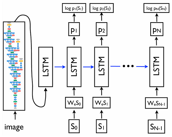
In fact, the main idea of the CPTR architecture is exactly the same as the earlier image captioning model, as both use the encoder-decoder structure. Previously, in the paper titled “Show and Tell: A Neural Image Caption Generator” [2], the models used are GoogLeNet (a.k.a. Inception V1) and LSTM for the two components, respectively. The illustration of the model proposed in the Show and Tell paper is shown in the following figure.
Despite having the same encoder-decoder structure, what makes CPTR different from the previous approach is the basis of the encoder and the decoder themselves. In CPTR, we combine the encoder part of the ViT (Vision Transformer) model with the decoder part of the original Transformer model. The use of transformer-based architecture for both components is essentially where the name CPTR comes from: CaPtion TransformeR.
Note that the discussions in this article are going to be highly related to ViT and Transformer, so I highly recommend you read my previous article about these two topics if you’re not yet familiar with them. You can find the links at the end of this article.
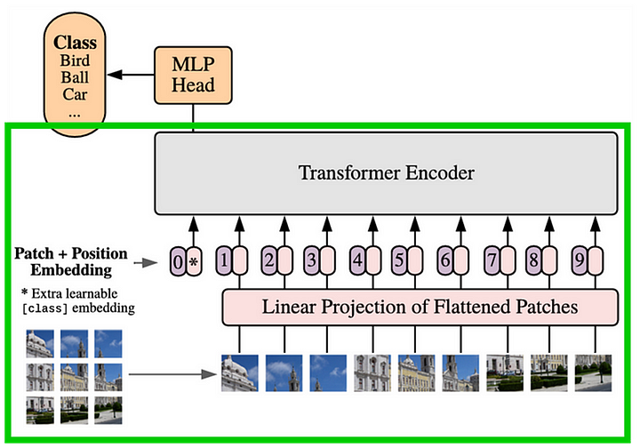
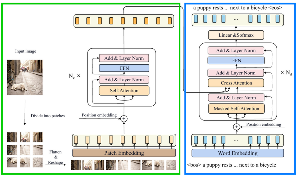
Figure 2 shows what the original ViT architecture looks like. Everything inside the green box is the encoder part of the architecture to be adopted as the CPTR encoder.
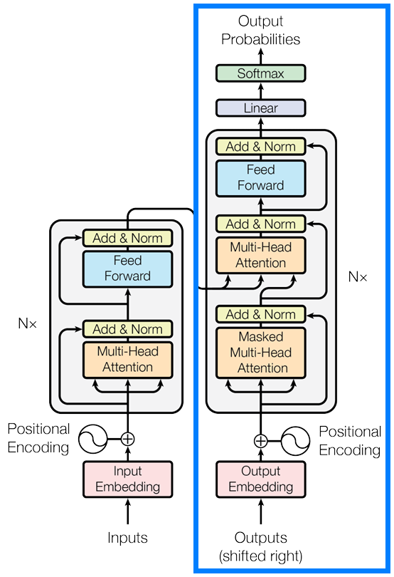
Next, Figure 3 displays the original Transformer architecture. The components enclosed in the blue box are the layers that we are going to implement in the CPTR decoder.
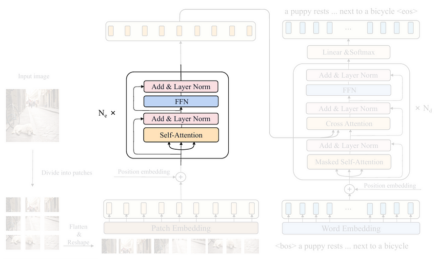
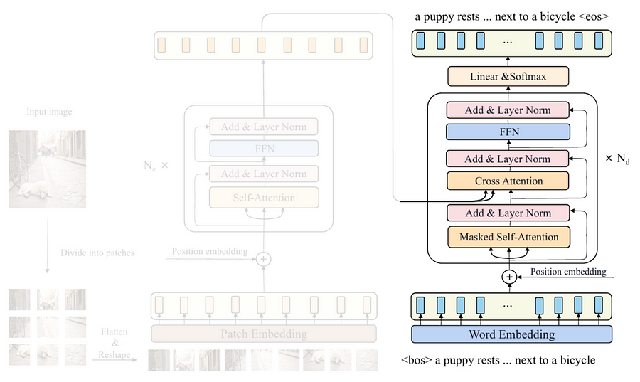
If we combine the components inside the green and blue boxes above, we are going to obtain the architecture shown in Figure 4 below. This is exactly what the CPTR model we are going to implement looks like. The idea here is that the ViT Encoder (green) works by encoding the input image into a specific tensor representation which will then be used as the basis of the Transformer Decoder (blue) to generate the corresponding caption.
That’s pretty much everything you need to know for now. I’ll explain more about the details as we go through the implementation.
Module imports & parameter configuration
As always, the first thing we need to do in the code is to import the required modules. In this case, we only import torch and torch.nn since we are about to implement the model from scratch.
# Codeblock 1
import torch
import torch.nn as nn
Next, we are going to initialize some parameters in Codeblock 2. If you have read my previous article about image captioning with GoogLeNet and LSTM, you’ll notice that here, we got a lot more parameters to initialize. In this article, I want to reproduce the CPTR model as closely as possible to the original one, so the parameters mentioned in the paper will be used in this implementation.
# Codeblock 2
BATCH_SIZE         = 1              #(1)

IMAGE_SIZE         = 384            #(2)
IN_CHANNELS        = 3              #(3)

SEQ_LENGTH         = 30             #(4)
VOCAB_SIZE         = 10000          #(5)

EMBED_DIM          = 768            #(6)
PATCH_SIZE         = 16             #(7)
NUM_PATCHES        = (IMAGE_SIZE//PATCH_SIZE) ** 2  #(8)
NUM_ENCODER_BLOCKS = 12             #(9)
NUM_DECODER_BLOCKS = 4              #(10)
NUM_HEADS          = 12             #(11)
HIDDEN_DIM         = EMBED_DIM * 4  #(12)
DROP_PROB          = 0.1            #(13)
The first parameter I want to explain is the BATCH_SIZE, which is written at the line marked with #(1). The number assigned to this variable is not quite important in our case since we are not actually going to train this model. This parameter is set to 1 because, by default, PyTorch treats input tensors as a batch of samples. Here I assume that we only have a single sample in a batch.
Next, remember that in the case of image captioning we are dealing with images and texts simultaneously. This essentially means that we need to set the parameters for the two. It is mentioned in the paper that the model accepts an RGB image of size 384×384 for the encoder input. Hence, we assign the values for IMAGE_SIZE and IN_CHANNELS variables based on this information (#(2) and #(3)). On the other hand, the paper does not mention the parameters for the captions. So, here I assume that the length of the caption is no more than 30 words (#(4)), with the vocabulary size estimated at 10000 unique words (#(5)).
The remaining parameters are related to the model configuration. Here we set the EMBED_DIM variable to 768 (#(6)). In the encoder side, this number indicates the length of the feature vector that represents each 16×16 image patch (#(7)). The same concept also applies to the decoder side, but in that case the feature vector will represent a single word in the caption. Talking more specifically about the PATCH_SIZE parameter, we are going to use the value to compute the total number of patches in the input image. Since the image has the size of 384×384, there will be 576 patches in total (#(8)).
When it comes to using an encoder-decoder architecture, it is possible to specify the number of encoder and decoder blocks to be used. Using more blocks typically allows the model to perform better in terms of the accuracy, yet in return, it will require more computational power. The authors of this paper decided to stack 12 encoder blocks (#(9)) and 4 decoder blocks (#(10)). Next, since CPTR is a transformer-based model, it is necessary to specify the number of attention heads within the attention blocks inside the encoders and the decoders, which in this case authors use 12 attention heads (#(11)). The value for the HIDDEN_DIM parameter is not mentioned anywhere in the paper. However, according to the ViT and the Transformer paper, this parameter is configured to be 4 times larger than EMBED_DIM (#(12)). The dropout rate is not mentioned in the paper either. Hence, I arbitrarily set DROP_PROB to 0.1 (#(13)).
Encoder
As the modules and parameters have been set up, now that we will get into the encoder part of the network. In this section we are going to implement and explain every single component inside the green box in Figure 4 one by one.
Patch embedding
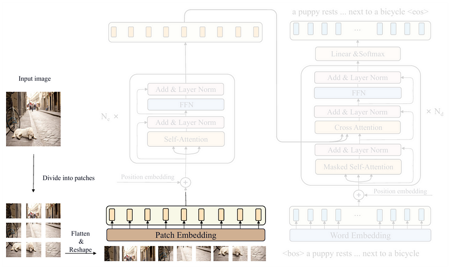
You can see in Figure 5 above that the first step to be done is dividing the input image into patches. This is essentially done because instead of focusing on local patterns like CNNs, ViT captures global context by learning the relationships between these patches. We can model this process with the Patcher class shown in the Codeblock 3 below. For the sake of simplicity, here I also include the process inside the patch embedding block within the same class.
# Codeblock 3
class Patcher(nn.Module):
   def __init__(self):
       super().__init__()

       #(1)
       self.unfold = nn.Unfold(kernel_size=PATCH_SIZE, stride=PATCH_SIZE)

       #(2)
       self.linear_projection = nn.Linear(in_features=IN_CHANNELS*PATCH_SIZE*PATCH_SIZE,
                                          out_features=EMBED_DIM)

   def forward(self, images):
       print(f'imagestt: {images.size()}')
       images = self.unfold(images)  #(3)
       print(f'after unfoldt: {images.size()}')

       images = images.permute(0, 2, 1)  #(4)
       print(f'after permutet: {images.size()}')

       features = self.linear_projection(images)  #(5)
       print(f'after lin projt: {features.size()}')

       return features
The patching itself is done using the nn.Unfold layer (#(1)). Here we need to set both the kernel_size and stride parameters to PATCH_SIZE (16) so that the resulting patches do not overlap with each other. This layer also automatically flattens these patches once it is applied to the input image. Meanwhile, the nn.Linear layer (#(2)) is employed to perform linear projection, i.e., the process done by the patch embedding block. By setting the out_features parameter to EMBED_DIM, this layer will map every single flattened patch into a feature vector of length 768.
The entire process should make more sense once you read the forward() method. You can see at line #(3) in the same codeblock that the input image is directly processed by the unfold layer. Next, we need to process the resulting tensor with the permute() method (#(4)) to swap the first and the second axis before feeding it to the linear_projection layer (#(5)). Additionally, here I also print out the tensor dimension after each layer so that you can better understand the transformation made at each step.
In order to check if our Patcher class works properly, we can just pass a dummy tensor through the network. Look at the Codeblock 4 below to see how I do it.
# Codeblock 4
patcher  = Patcher()

images   = torch.randn(BATCH_SIZE, IN_CHANNELS, IMAGE_SIZE, IMAGE_SIZE)
features = patcher(images)
# Codeblock 4 Output
images : torch.Size([1, 3, 384, 384])
after unfold : torch.Size([1, 768, 576]) #(1)
after permute : torch.Size([1, 576, 768]) #(2)
after lin proj : torch.Size([1, 576, 768]) #(3)The tensor I passed above represents an RGB image of size 384×384. Here we can see that after the unfold operation is performed, the tensor dimension changed to 1×768×576 (#(1)), denoting the flattened 3×16×16 patch for each of the 576 patches. Unfortunately, this output shape does not match what we need. Remember that in ViT, we perceive image patches as a sequence, so we need to swap the 1st and 2nd axes because typically, the 1st dimension of a tensor represents the temporal axis, while the 2nd one represents the feature vector of each timestep. As the permute() operation is performed, our tensor is now having the dimension of 1×576×768 (#(2)). Lastly, we pass this tensor through the linear projection layer, which the resulting tensor shape remains the same since we set the EMBED_DIM parameter to the same size (768) (#(3)). Despite having the same dimension, the information contained in the final tensor should be richer thanks to the transformation applied by the trainable weights of the linear projection layer.
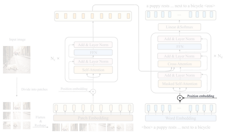
Learnable positional embedding
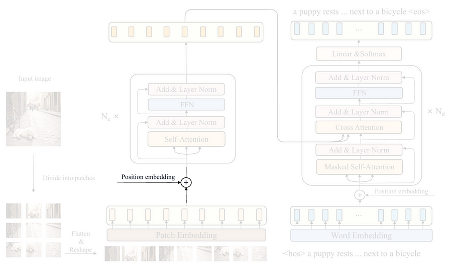
After the input image has successfully been converted into a sequence of patches, the next thing to do is to inject the so-called positional embedding tensor. This is essentially done because a transformer without positional embedding is permutation-invariant, meaning that it treats the input sequence as if their order does not matter. Interestingly, since an image is not a literal sequence, we should set the positional embedding to be learnable such that it will be able to somewhat reorder the patch sequence that it thinks works best in representing the spatial information. However, keep in mind that the term “reordering” here does not mean that we physically rearrange the sequence. Rather, it does so by adjusting the embedding weights.
The implementation is pretty simple. All we need to do is just to initialize a tensor using nn.Parameter which the dimension is set to match with the output from the Patcher model, i.e., 576×768. Also, don’t forget to write requires_grad=True just to ensure that the tensor is trainable. Look at the Codeblock 5 below for the details.
# Codeblock 5
class LearnableEmbedding(nn.Module):
   def __init__(self):
       super().__init__()
       self.learnable_embedding = nn.Parameter(torch.randn(size=(NUM_PATCHES, EMBED_DIM)),
                                               requires_grad=True)

   def forward(self):
       pos_embed = self.learnable_embedding
       print(f'learnable embeddingt: {pos_embed.size()}')

       return pos_embed
Now let’s run the following codeblock to see whether our LearnableEmbedding class works properly. You can see in the printed output that it successfully created the positional embedding tensor as expected.
# Codeblock 6
learnable_embedding = LearnableEmbedding()

pos_embed = learnable_embedding()
# Codeblock 6 Output
learnable embedding : torch.Size([576, 768])The main encoder block
The next thing we are going to do is to construct the main encoder block displayed in the Figure 7 above. Here you can see that this block consists of several sub-components, namely self-attention, layer norm, FFN (Feed-Forward Network), and another layer norm. The Codeblock 7a below shows how I initialize these layers inside the __init__() method of the EncoderBlock class.
# Codeblock 7a
class EncoderBlock(nn.Module):
   def __init__(self):
       super().__init__()

       #(1)
       self.self_attention = nn.MultiheadAttention(embed_dim=EMBED_DIM,
                                                   num_heads=NUM_HEADS,
                                                   batch_first=True,  #(2)
                                                   dropout=DROP_PROB)

       self.layer_norm_0 = nn.LayerNorm(EMBED_DIM)  #(3)

       self.ffn = nn.Sequential(  #(4)
           nn.Linear(in_features=EMBED_DIM, out_features=HIDDEN_DIM),
           nn.GELU(),
           nn.Dropout(p=DROP_PROB),
           nn.Linear(in_features=HIDDEN_DIM, out_features=EMBED_DIM),
       )

       self.layer_norm_1 = nn.LayerNorm(EMBED_DIM)  #(5)
I’ve previously mentioned that the idea of ViT is to capture the relationships between patches within an image. This process is done by the multihead attention layer I initialize at line #(1) in the above codeblock. One thing to keep in mind here is that we need to set the batch_first parameter to True (#(2)). This is essentially done so that the attention layer will be compatible with our tensor shape, in which the batch dimension (batch_size) is at the 0th axis of the tensor. Next, the two layer normalization layers need to be initialized separately, as shown at line #(3) and #(5). Lastly, we initialize the FFN block at line #(4), which the layers stacked using nn.Sequential follows the structure defined in the following equation.

As the __init__() method is complete, we will now continue with the forward() method. Let’s take a look at the Codeblock 7b below.
# Codeblock 7b
   def forward(self, features):  #(1)

       residual = features  #(2)
       print(f'features & residualt: {residual.size()}')

       #(3)
       features, self_attn_weights = self.self_attention(query=features,
                                                         key=features,
                                                         value=features)
       print(f'after self attentiont: {features.size()}')
       print(f"self attn weightst: {self_attn_weights.shape}")

       features = self.layer_norm_0(features + residual)  #(4)
       print(f'after normtt: {features.size()}')


       residual = features
       print(f'nfeatures & residualt: {residual.size()}')

       features = self.ffn(features)  #(5)
       print(f'after ffntt: {features.size()}')

       features = self.layer_norm_1(features + residual)
       print(f'after normtt: {features.size()}')

       return features
Here you can see that the input tensor is named features (#(1)). I name it this way because the input of the EncoderBlock is the image that has already been processed with Patcher and LearnableEmbedding, instead of a raw image. Before doing anything, notice in the encoder block that there is a branch separated from the main flow which then returns back to the normalization layer. This branch is commonly known as a residual connection. To implement this, we need to store the original input tensor to the residual variable as I demonstrate at line #(2). As the input tensor has been copied, now we are ready to process the original input with the multihead attention layer (#(3)). Since this is a self-attention (not a cross-attention), the query, key, and value inputs for this layer are all derived from the features tensor. Next, the layer normalization operation is then performed at line #(4), which the input for this layer already contains information from the attention block as well as the residual connection. The remaining steps are basically the same as what I just explained, except that here we replace the self-attention block with FFN (#(5)).
In the following codeblock, I’ll test the EncoderBlock class by passing a dummy tensor of size 1×576×768, simulating an output tensor from the previous operations.
# Codeblock 8
encoder_block = EncoderBlock()

features = torch.randn(BATCH_SIZE, NUM_PATCHES, EMBED_DIM)
features = encoder_block(features)
Below is what the tensor dimension looks like throughout the entire process inside the model.
# Codeblock 8 Output
features & residual  : torch.Size([1, 576, 768])  #(1)
after self attention : torch.Size([1, 576, 768])
self attn weights    : torch.Size([1, 576, 576])  #(2)
after norm           : torch.Size([1, 576, 768])

features & residual  : torch.Size([1, 576, 768])
after ffn            : torch.Size([1, 576, 768])  #(3)
after norm           : torch.Size([1, 576, 768])  #(4)
Here you can see that the final output tensor (#(4)) has the same size as the input (#(1)), allowing us to stack multiple encoder blocks without having to worry about messing up the tensor dimensions. Not only that, the size of the tensor also appears to be unchanged from the beginning all the way to the last layer. In fact, there are actually lots of transformations performed inside the attention block, but we just can’t see it since the entire process is done internally by the nn.MultiheadAttention layer. One of the tensors produced in the layer that we can observe is the attention weight (#(2)). This weight matrix, which has the size of 576×576, is responsible for storing information regarding the relationships between one patch and every other patch in the image. Furthermore, changes in tensor dimension actually also happened inside the FFN layer. The feature vector of each patch which has the initial length of 768 changed to 3072 and immediately shrunk back to 768 again (#(3)). However, this transformation is not printed since the process is wrapped with nn.Sequential back at line #(4) in Codeblock 7a.
ViT encoder

As we have finished implementing all encoder components, now that we will assemble them to construct the actual ViT Encoder. We are going to do it in the Encoder class in Codeblock 9.
# Codeblock 9
class Encoder(nn.Module):
   def __init__(self):
       super().__init__()
       self.patcher = Patcher()  #(1)
       self.learnable_embedding = LearnableEmbedding()  #(2)

       #(3)
       self.encoder_blocks = nn.ModuleList(EncoderBlock() for _ in range(NUM_ENCODER_BLOCKS))

   def forward(self, images):  #(4)
       print(f'imagesttt: {images.size()}')

       features = self.patcher(images)  #(5)
       print(f'after patchertt: {features.size()}')

       features = features + self.learnable_embedding()  #(6)
       print(f'after learn embedt: {features.size()}')

       for i, encoder_block in enumerate(self.encoder_blocks):
           features = encoder_block(features)  #(7)
           print(f"after encoder block #{i}t: {features.shape}")

       return features
Inside the __init__() method, what we need to do is to initialize all components we created earlier, i.e., Patcher (#(1)), LearnableEmbedding (#(2)), and EncoderBlock (#(3)). In this case, the EncoderBlock is initialized inside nn.ModuleList since we want to repeat it NUM_ENCODER_BLOCKS (12) times. To the forward() method, it initially works by accepting raw image as the input (#(4)). We then process it with the patcher layer (#(5)) to divide the image into small patches and transform them with the linear projection operation. The learnable positional embedding tensor is then injected into the resulting output by element-wise addition (#(6)). Lastly, we pass it into the 12 encoder blocks sequentially with a simple for loop (#(7)).
Now, in Codeblock 10, I am going to pass a dummy image through the entire encoder. Note that since I want to focus on the flow of this Encoder class, I re-run the previous classes we created earlier with the print() functions commented out so that the outputs will look neat.
# Codeblock 10
encoder = Encoder()

images = torch.randn(BATCH_SIZE, IN_CHANNELS, IMAGE_SIZE, IMAGE_SIZE)
features = encoder(images)
And below is what the flow of the tensor looks like. Here, we can see that our dummy input image successfully passed through all layers in the network, including the encoder blocks that we repeat 12 times. The resulting output tensor is now context-aware, meaning that it already contains information about the relationships between patches within the image. Therefore, this tensor is now ready to be processed further with the decoder, which will later be discussed in the subsequent section.
# Codeblock 10 Output
images                  : torch.Size([1, 3, 384, 384])
after patcher           : torch.Size([1, 576, 768])
after learn embed       : torch.Size([1, 576, 768])
after encoder block #0  : torch.Size([1, 576, 768])
after encoder block #1  : torch.Size([1, 576, 768])
after encoder block #2  : torch.Size([1, 576, 768])
after encoder block #3  : torch.Size([1, 576, 768])
after encoder block #4  : torch.Size([1, 576, 768])
after encoder block #5  : torch.Size([1, 576, 768])
after encoder block #6  : torch.Size([1, 576, 768])
after encoder block #7  : torch.Size([1, 576, 768])
after encoder block #8  : torch.Size([1, 576, 768])
after encoder block #9  : torch.Size([1, 576, 768])
after encoder block #10 : torch.Size([1, 576, 768])
after encoder block #11 : torch.Size([1, 576, 768])
ViT encoder (alternative)
I want to show you something before we talk about the decoder. If you think that our approach above is too complicated, it is actually possible for you to use nn.TransformerEncoderLayer from PyTorch so that you don’t need to implement the EncoderBlock class from scratch. To do so, I am going to reimplement the Encoder class, but this time I’ll name it EncoderTorch.
# Codeblock 11
class EncoderTorch(nn.Module):
   def __init__(self):
       super().__init__()
       self.patcher = Patcher()
       self.learnable_embedding = LearnableEmbedding()

       #(1)
       encoder_block = nn.TransformerEncoderLayer(d_model=EMBED_DIM,
                                                  nhead=NUM_HEADS,
                                                  dim_feedforward=HIDDEN_DIM,
                                                  dropout=DROP_PROB,
                                                  batch_first=True)

       #(2)
       self.encoder_blocks = nn.TransformerEncoder(encoder_layer=encoder_block,
                                                   num_layers=NUM_ENCODER_BLOCKS)

   def forward(self, images):
       print(f'imagesttt: {images.size()}')

       features = self.patcher(images)
       print(f'after patchertt: {features.size()}')

       features = features + self.learnable_embedding()
       print(f'after learn embedt: {features.size()}')

       features = self.encoder_blocks(features)  #(3)
       print(f'after encoder blockst: {features.size()}')

       return features
What we basically do in the above codeblock is that instead of using the EncoderBlock class, here we use nn.TransformerEncoderLayer (#(1)), which will automatically create a single encoder block based on the parameters we pass to it. To repeat it multiple times, we can just use nn.TransformerEncoder and pass a number to the num_layers parameter (#(2)). With this approach, we don’t necessarily need to write the forward pass in a loop like what we did earlier (#(3)).
The testing code in the Codeblock 12 below is exactly the same as the one in Codeblock 10, except that here I use the EncoderTorch class. You can also see here that the output is basically the same as the previous one.
# Codeblock 12
encoder_torch = EncoderTorch()

images = torch.randn(BATCH_SIZE, IN_CHANNELS, IMAGE_SIZE, IMAGE_SIZE)
features = encoder_torch(images)
# Codeblock 12 Output
images : torch.Size([1, 3, 384, 384])
after patcher : torch.Size([1, 576, 768])
after learn embed : torch.Size([1, 576, 768])
after encoder blocks : torch.Size([1, 576, 768])Decoder
As we have successfully created the encoder part of the CPTR architecture, now that we will talk about the decoder. In this section I am going to implement every single component inside the blue box in Figure 4. Based on the figure, we can see that the decoder accepts two inputs, i.e., the image caption ground truth (the lower part of the blue box) and the sequence of embedded patches produced by the encoder (the arrow coming from the green box). It is important to know that the architecture drawn in Figure 4 is intended to illustrate the training phase, where the entire caption ground truth is fed into the decoder. Later in the inference phase, we only provide a (Beginning of Sentence) token for the caption input. The decoder will then predict each word sequentially based on the given image and the previously generated words. This process is commonly known as an autoregressive mechanism.
Sinusoidal positional embedding
If you take a look at the CPTR model, you’ll see that the first step in the decoder is to convert each word into the corresponding feature vector representation using the word embedding block. However, since this step is very easy, we are going to implement it later. Now let’s assume that this word vectorization process is already done, so we can move to the positional embedding part.
As I’ve mentioned earlier, since transformer is permutation-invariant by nature, we need to apply positional embedding to the input sequence. Different from the previous one, here we use the so-called sinusoidal positional embedding. We can think of it like a method to label each word vector by assigning numbers obtained from a sinusoidal wave. By doing so, we can expect our model to understand word orders thanks to the information given by the wave patterns.
If you go back to Codeblock 6 Output, you’ll see that the positional embedding tensor in the encoder has the size of NUM_PATCHES × EMBED_DIM (576×768). What we basically want to do in the decoder is to create a tensor having the size of SEQ_LENGTH × EMBED_DIM (30×768), which the values are computed based on the equation shown in Figure 11. This tensor is then set to be non-trainable because a sequence of words must maintain a fixed order to preserve its meaning.

Here I want to explain the following code quickly because I actually have discussed this more thoroughly in my previous article about Transformer. Generally speaking, what we basically do here is to create the sine and cosine wave using torch.sin() (#(1)) and torch.cos() (#(2)). The resulting two tensors are then merged using the code at line #(3) and #(4).
# Codeblock 13
class SinusoidalEmbedding(nn.Module):
   def forward(self):
       pos = torch.arange(SEQ_LENGTH).reshape(SEQ_LENGTH, 1)
       print(f"postt: {pos.shape}")

       i = torch.arange(0, EMBED_DIM, 2)
       denominator = torch.pow(10000, i/EMBED_DIM)
       print(f"denominatort: {denominator.shape}")

       even_pos_embed = torch.sin(pos/denominator)  #(1)
       odd_pos_embed  = torch.cos(pos/denominator)  #(2)
       print(f"even_pos_embedt: {even_pos_embed.shape}")

       stacked = torch.stack([even_pos_embed, odd_pos_embed], dim=2)  #(3)
       print(f"stackedtt: {stacked.shape}")

       pos_embed = torch.flatten(stacked, start_dim=1, end_dim=2)  #(4)
       print(f"pos_embedt: {pos_embed.shape}")

       return pos_embed
Now we can check if the SinusoidalEmbedding class above works properly by running the Codeblock 14 below. As expected earlier, here you can see that the resulting tensor has the size of 30×768. This dimension matches with the tensor obtained by the process done in the word embedding block, allowing them to be summed in an element-wise manner.
# Codeblock 14
sinusoidal_embedding = SinusoidalEmbedding()
pos_embed = sinusoidal_embedding()
# Codeblock 14 Output
pos : torch.Size([30, 1])
denominator : torch.Size([384])
even_pos_embed : torch.Size([30, 384])
stacked : torch.Size([30, 384, 2])
pos_embed : torch.Size([30, 768])Look-ahead mask
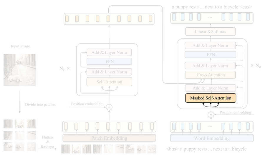
The next thing I am going to talk about in the decoder is the masked self-attention layer highlighted in the above figure. I am not going to code the attention mechanism from scratch. Rather, I’ll only implement the so-called look-ahead mask, which will be useful for the self-attention layer so that it doesn’t attend to the subsequent words in the caption during the training phase.
The way to do it is pretty easy, what we need to do is just to create a triangular matrix which the size is set to match with the attention weight matrix, i.e., SEQ_LENGTH × SEQ_LENGTH (30×30). Look at the create_mask()function below for the details.
# Codeblock 15
def create_mask(seq_length):
   mask = torch.tril(torch.ones((seq_length, seq_length)))  #(1)
   mask[mask == 0] = -float('inf')  #(2)
   mask[mask == 1] = 0  #(3)
   return mask
Even though creating a triangular matrix can simply be done with torch.tril() and torch.ones() (#(1)), but here we need to make a little modification by changing the 0 values to -inf (#(2)) and the 1s to 0 (#(3)). This is essentially done because the nn.MultiheadAttention layer applies the mask by element-wise addition. By assigning -inf to the subsequent words, the attention mechanism will completely ignore them. Again, the internal process inside an attention layer has also been discussed in detail in my previous article about transformer.
Now I am going to run the function with seq_length=7 so that you can see what the mask actually looks like. Later in the complete flow, we need to set the seq_length parameter to SEQ_LENGTH (30) so that it matches with the actual caption length.
# Codeblock 16
mask_example = create_mask(seq_length=7)
mask_example
# Codeblock 16 Output
tensor([[0., -inf, -inf, -inf, -inf, -inf, -inf],
[0., 0., -inf, -inf, -inf, -inf, -inf],
[0., 0., 0., -inf, -inf, -inf, -inf],
[0., 0., 0., 0., -inf, -inf, -inf],
[0., 0., 0., 0., 0., -inf, -inf],
[0., 0., 0., 0., 0., 0., -inf],
[0., 0., 0., 0., 0., 0., 0.]])The main decoder block
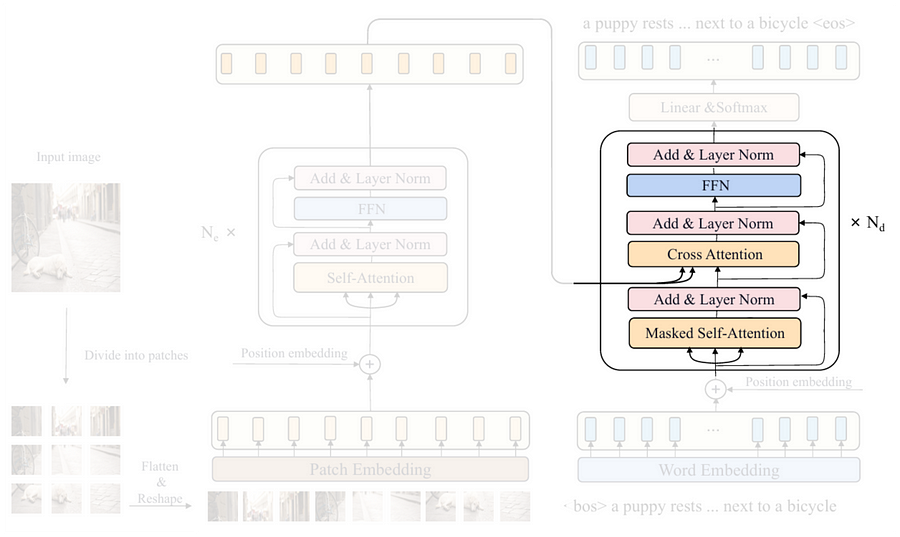
We can see in the above figure that the structure of the decoder block is a bit longer than that of the encoder block. It seems like everything is nearly the same, except that the decoder part has a cross-attention mechanism and an additional layer normalization step placed after it. This cross-attention layer can actually be perceived as the bridge between the encoder and the decoder, as it is employed to capture the relationships between each word in the caption and every single patch in the input image. The two arrows coming from the encoder are the key and value inputs for the attention layer, whereas the query is derived from the previous layer in the decoder itself. Look at the Codeblock 17a and 17b below to see the implementation of the entire decoder block.
# Codeblock 17a
class DecoderBlock(nn.Module):
   def __init__(self):
       super().__init__()

       #(1)
       self.self_attention = nn.MultiheadAttention(embed_dim=EMBED_DIM,
                                                   num_heads=NUM_HEADS,
                                                   batch_first=True,
                                                   dropout=DROP_PROB)
       #(2)
       self.layer_norm_0 = nn.LayerNorm(EMBED_DIM)
       #(3)
       self.cross_attention = nn.MultiheadAttention(embed_dim=EMBED_DIM,
                                                    num_heads=NUM_HEADS,
                                                    batch_first=True,
                                                    dropout=DROP_PROB)

       #(4)
       self.layer_norm_1 = nn.LayerNorm(EMBED_DIM)

       #(5)
       self.ffn = nn.Sequential(
           nn.Linear(in_features=EMBED_DIM, out_features=HIDDEN_DIM),
           nn.GELU(),
           nn.Dropout(p=DROP_PROB),
           nn.Linear(in_features=HIDDEN_DIM, out_features=EMBED_DIM),
       )

       #(6)
       self.layer_norm_2 = nn.LayerNorm(EMBED_DIM)
In the __init__() method, we first initialize both self-attention (#(1)) and cross-attention (#(3)) layers with nn.MultiheadAttention. These two layers appear to be exactly the same now, but later you’ll see the difference in the forward() method. The three layer normalization operations are initialized separately as shown at line #(2), #(4) and #(6), since each of them will contain different normalization parameters. Lastly, the ffn layer (#(5)) is exactly the same as the one in the encoder, which basically follows the equation back in Figure 8.
Talking about the forward() method below, it initially works by accepting three inputs: features, captions, and attn_mask, which each of them denotes the tensor coming from the encoder, the tensor from the decoder itself, and a look-ahead mask, respectively (#(1)). The remaining steps are somewhat similar to that of the EncoderBlock, except that here we repeat the multihead attention block twice. The first attention mechanism takes captions as the query, key, and value parameters (#(2)). This is essentially done because we want the layer to capture the context within the captions tensor itself — hence the name self-attention. Here we also need to pass the attn_mask parameter to this layer so that it cannot see the subsequent words during the training phase. The second attention mechanism is different (#(3)). Since we want to combine the information from the encoder and the decoder, we need to pass the captions tensor as the query, whereas the features tensor will be passed as the key and value — hence the name cross-attention. A look-ahead mask is not necessary in the cross-attention layer since later in the inference phase the model will be able to see the entire input image at once rather than looking at the patches one by one. As the tensor has been processed by the two attention layers, we will then pass it through the feed forward network (#(4)). Lastly, don’t forget to create the residual connections and apply the layer normalization steps after each sub-component.
# Codeblock 17b
   def forward(self, features, captions, attn_mask):  #(1)
       print(f"attn_masktt: {attn_mask.shape}")
       residual = captions
       print(f"captions & residualt: {captions.shape}")

       #(2)
       captions, self_attn_weights = self.self_attention(query=captions,
                                                         key=captions,
                                                         value=captions,
                                                         attn_mask=attn_mask)
       print(f"after self attentiont: {captions.shape}")
       print(f"self attn weightst: {self_attn_weights.shape}")

       captions = self.layer_norm_0(captions + residual)
       print(f"after normtt: {captions.shape}")


       print(f"nfeaturestt: {features.shape}")
       residual = captions
       print(f"captions & residualt: {captions.shape}")

       #(3)
       captions, cross_attn_weights = self.cross_attention(query=captions,
                                                           key=features,
                                                           value=features)
       print(f"after cross attentiont: {captions.shape}")
       print(f"cross attn weightst: {cross_attn_weights.shape}")

       captions = self.layer_norm_1(captions + residual)
       print(f"after normtt: {captions.shape}")

       residual = captions
       print(f"ncaptions & residualt: {captions.shape}")

       captions = self.ffn(captions)  #(4)
       print(f"after ffntt: {captions.shape}")

       captions = self.layer_norm_2(captions + residual)
       print(f"after normtt: {captions.shape}")

       return captions
As the DecoderBlock class is completed, we can now test it with the following code.
# Codeblock 18
decoder_block = DecoderBlock()

features = torch.randn(BATCH_SIZE, NUM_PATCHES, EMBED_DIM)  #(1)
captions = torch.randn(BATCH_SIZE, SEQ_LENGTH, EMBED_DIM)   #(2)
look_ahead_mask = create_mask(seq_length=SEQ_LENGTH)  #(3)

captions = decoder_block(features, captions, look_ahead_mask)
Here we assume that features is a tensor containing a sequence of patch embeddings produced by the encoder (#(1)), while captions is a sequence of embedded words (#(2)). The seq_length parameter of the look-ahead mask is set to SEQ_LENGTH (30) to match it to the number of words in the caption (#(3)). The tensor dimensions after each step are displayed in the following output.
# Codeblock 18 Output
attn_mask             : torch.Size([30, 30])
captions & residual   : torch.Size([1, 30, 768])
after self attention  : torch.Size([1, 30, 768])
self attn weights     : torch.Size([1, 30, 30])    #(1)
after norm            : torch.Size([1, 30, 768])

features              : torch.Size([1, 576, 768])
captions & residual   : torch.Size([1, 30, 768])
after cross attention : torch.Size([1, 30, 768])
cross attn weights    : torch.Size([1, 30, 576])   #(2)
after norm            : torch.Size([1, 30, 768])

captions & residual   : torch.Size([1, 30, 768])
after ffn             : torch.Size([1, 30, 768])
after norm            : torch.Size([1, 30, 768])
Here we can see that our DecoderBlock class works properly as it successfully processed the input tensors all the way to the last layer in the network. Here I want you to take a closer look at the attention weights at lines #(1) and #(2). Based on these two lines, we can confirm that our decoder implementation is correct since the attention weight produced by the self-attention layer has the size of 30×30 (#(1)), which basically means that this layer really captured the context within the input caption. Meanwhile, the attention weight matrix generated by the cross-attention layer has the size of 30×576 (#(2)), indicating that it successfully captured the relationships between the words and the patches. This essentially implies that after cross-attention operation is performed, the resulting captions tensor has been enriched with the information from the image.
Transformer decoder
Now that we have successfully created all components for the entire decoder, what I am going to do next is to put them together into a single class. Look at the Codeblock 19a and 19b below to see how I do that.
# Codeblock 19a
class Decoder(nn.Module):
   def __init__(self):
       super().__init__()

       #(1)
       self.embedding = nn.Embedding(num_embeddings=VOCAB_SIZE,
                                     embedding_dim=EMBED_DIM)

       #(2)
       self.sinusoidal_embedding = SinusoidalEmbedding()

       #(3)
       self.decoder_blocks = nn.ModuleList(DecoderBlock() for _ in range(NUM_DECODER_BLOCKS))

       #(4)
       self.linear = nn.Linear(in_features=EMBED_DIM,
                               out_features=VOCAB_SIZE)
If you compare this Decoder class with the Encoder class from codeblock 9, you’ll notice that they are somewhat similar in terms of the structure. In the encoder, we convert image patches into vectors using Patcher, while in the decoder we convert every single word in the caption into a vector using the nn.Embedding layer (#(1)), which I haven’t explained earlier. Afterward, we initialize the positional embedding layer, where for the decoder we use the sinusoidal rather than the trainable one (#(2)). Next, we stack multiple decoder blocks using nn.ModuleList (#(3)). The linear layer written at line #(4), which doesn’t exist in the encoder, is necessary to be implemented here since it will be responsible to map each of the embedded words into a vector of length VOCAB_SIZE (10000). Later on, this vector will contain the logit of every word in the dictionary, and what we need to do afterward is just to take the index containing the highest value, i.e., the most likely word to be predicted.
The flow of the tensors within the forward() method itself is also pretty similar to the one in the Encoder class. In the Codeblock 19b below we pass features, captions, and attn_mask as the input (#(1)). Keep in mind that in this case the captions tensor contains the raw word sequence, so we need to vectorize these words with the embedding layer beforehand (#(2)). Next, we inject the sinusoidal positional embedding tensor using the code at line #(3) before eventually passing it through the four decoder blocks sequentially (#(4)). Finally, we pass the resulting tensor through the last linear layer to obtain the prediction logits (#(5)).
# Codeblock 19b
   def forward(self, features, captions, attn_mask):  #(1)
       print(f"featurestt: {features.shape}")
       print(f"captionstt: {captions.shape}")

       captions = self.embedding(captions)  #(2)
       print(f"after embeddingtt: {captions.shape}")

       captions = captions + self.sinusoidal_embedding()  #(3)
       print(f"after sin embedtt: {captions.shape}")

       for i, decoder_block in enumerate(self.decoder_blocks):
           captions = decoder_block(features, captions, attn_mask)  #(4)
           print(f"after decoder block #{i}t: {captions.shape}")

       captions = self.linear(captions)  #(5)
       print(f"after lineartt: {captions.shape}")

       return captions
At this point you might be wondering why we don’t implement the softmax activation function as drawn in the illustration. This is essentially because during the training phase, softmax is typically included within the loss function, whereas in the inference phase, the index of the largest value will remain the same regardless of whether softmax is applied.
Now let’s run the following testing code to check whether there are errors in our implementation. Previously I mentioned that the captions input of the Decoder class is a raw word sequence. To simulate this, we can simply create a sequence of random integers ranging between 0 and VOCAB_SIZE (10000) with the length of SEQ_LENGTH (30) words (#(1)).
# Codeblock 20
decoder = Decoder()

features = torch.randn(BATCH_SIZE, NUM_PATCHES, EMBED_DIM)
captions = torch.randint(0, VOCAB_SIZE, (BATCH_SIZE, SEQ_LENGTH))  #(1)

captions = decoder(features, captions, look_ahead_mask)
And below is what the resulting output looks like. Here you can see in the last line that the linear layer produced a tensor of size 30×10000, indicating that our decoder model is now capable of predicting the logit scores for each word in the vocabulary across all 30 sequence positions.
# Codeblock 20 Output
features               : torch.Size([1, 576, 768])
captions               : torch.Size([1, 30])
after embedding        : torch.Size([1, 30, 768])
after sin embed        : torch.Size([1, 30, 768])
after decoder block #0 : torch.Size([1, 30, 768])
after decoder block #1 : torch.Size([1, 30, 768])
after decoder block #2 : torch.Size([1, 30, 768])
after decoder block #3 : torch.Size([1, 30, 768])
after linear           : torch.Size([1, 30, 10000])
Transformer decoder (alternative)
It is actually also possible to make the code simpler by replacing the DecoderBlock class with the nn.TransformerDecoderLayer, just like what we did in the ViT Encoder. Below is what the code looks like if we use this approach instead.
# Codeblock 21
class DecoderTorch(nn.Module):
   def __init__(self):
       super().__init__()
       self.embedding = nn.Embedding(num_embeddings=VOCAB_SIZE,
                                     embedding_dim=EMBED_DIM)

       self.sinusoidal_embedding = SinusoidalEmbedding()

       #(1)
       decoder_block = nn.TransformerDecoderLayer(d_model=EMBED_DIM,
                                                  nhead=NUM_HEADS,
                                                  dim_feedforward=HIDDEN_DIM,
                                                  dropout=DROP_PROB,
                                                  batch_first=True)

       #(2)
       self.decoder_blocks = nn.TransformerDecoder(decoder_layer=decoder_block,
                                                   num_layers=NUM_DECODER_BLOCKS)

       self.linear = nn.Linear(in_features=EMBED_DIM,
                               out_features=VOCAB_SIZE)

   def forward(self, features, captions, tgt_mask):
       print(f"featurestt: {features.shape}")
       print(f"captionstt: {captions.shape}")

       captions = self.embedding(captions)
       print(f"after embeddingtt: {captions.shape}")

       captions = captions + self.sinusoidal_embedding()
       print(f"after sin embedtt: {captions.shape}")

       #(3)
       captions = self.decoder_blocks(tgt=captions,
                                      memory=features,
                                      tgt_mask=tgt_mask)
       print(f"after decoder blockst: {captions.shape}")

       captions = self.linear(captions)
       print(f"after lineartt: {captions.shape}")

       return captions
The main difference you will see in the __init__() method is the use of nn.TransformerDecoderLayer and nn.TransformerDecoder at line #(1) and #(2), where the former is used to initialize a single decoder block, and the latter is for repeating the block multiple times. Next, the forward() method is mostly similar to the one in the Decoder class, except that the forward propagation on the decoder blocks is automatically repeated four times without needing to be put inside a loop (#(3)). One thing that you need to pay attention to in the decoder_blocks layer is that the tensor coming from the encoder (features) must be passed as the argument for the memory parameter. Meanwhile, the tensor from the decoder itself (captions) has to be passed as the input to the tgt parameter.
The testing code for the DecoderTorch model below is basically the same as the one written in Codeblock 20. Here you can see that this model also generates the final output tensor of size 30×10000.
# Codeblock 22
decoder_torch = DecoderTorch()

features = torch.randn(BATCH_SIZE, NUM_PATCHES, EMBED_DIM)
captions = torch.randint(0, VOCAB_SIZE, (BATCH_SIZE, SEQ_LENGTH))

captions = decoder_torch(features, captions, look_ahead_mask)
# Codeblock 22 Output
features : torch.Size([1, 576, 768])
captions : torch.Size([1, 30])
after embedding : torch.Size([1, 30, 768])
after sin embed : torch.Size([1, 30, 768])
after decoder blocks : torch.Size([1, 30, 768])
after linear : torch.Size([1, 30, 10000])The entire CPTR model
Finally, it’s time to put the encoder and the decoder part we just created into a single class to actually construct the CPTR architecture. You can see in Codeblock 23 below that the implementation is very simple. All we need to do here is just to initialize the encoder (#(1)) and the decoder (#(2)) components, then pass the raw images and the corresponding caption ground truths as well as the look-ahead mask to the forward() method (#(3)). Additionally, it is also possible for you to replace the Encoder and the Decoder with EncoderTorch and DecoderTorch, respectively.
# Codeblock 23
class EncoderDecoder(nn.Module):
   def __init__(self):
       super().__init__()
       self.encoder = Encoder()  #EncoderTorch()  #(1)
       self.decoder = Decoder()  #DecoderTorch()  #(2)

   def forward(self, images, captions, look_ahead_mask):  #(3)
       print(f"imagesttt: {images.shape}")
       print(f"captionstt: {captions.shape}")

       features = self.encoder(images)
       print(f"after encodertt: {features.shape}")

       captions = self.decoder(features, captions, look_ahead_mask)
       print(f"after decodertt: {captions.shape}")

       return captions
We can do the testing by passing dummy tensors through it. See the Codeblock 24 below for the details. In this case, images is basically just a tensor of random numbers having the dimension of 1×3×384×384 (#(1)), while captions is a tensor of size 1×30 containing random integers (#(2)).
# Codeblock 24
encoder_decoder = EncoderDecoder()

images = torch.randn(BATCH_SIZE, IN_CHANNELS, IMAGE_SIZE, IMAGE_SIZE)  #(1)
captions = torch.randint(0, VOCAB_SIZE, (BATCH_SIZE, SEQ_LENGTH))  #(2)

captions = encoder_decoder(images, captions, look_ahead_mask)
Below is what the output looks like. We can see here that our input images and captions successfully went through all layers in the network, which basically means that the CPTR model we created is now ready to actually be trained on image captioning datasets.
# Codeblock 24 Output
images         : torch.Size([1, 3, 384, 384])
captions       : torch.Size([1, 30])
after encoder  : torch.Size([1, 576, 768])
after decoder  : torch.Size([1, 30, 10000])
Ending
That was pretty much everything about the theory and implementation of the CaPtion TransformeR architecture. Let me know what deep learning architecture I should implement next. Feel free to leave a comment if you spot any mistakes in this article!
The code used in this article is available in my GitHub repo. Here’s the link to my previous article about image captioning, Vision Transformer (ViT), and the original Transformer.
References
[1] Wei Liu et al. CPTR: Full Transformer Network for Image Captioning. Arxiv. https://arxiv.org/pdf/2101.10804 [Accessed November 16, 2024].
[2] Oriol Vinyals et al. Show and Tell: A Neural Image Caption Generator. Arxiv. https://arxiv.org/pdf/1411.4555 [Accessed December 3, 2024].
[3] Image originally created by author based on: Alexey Dosovitskiy et al. An Image is Worth 16×16 Words: Transformers for Image Recognition at Scale. Arxiv. https://arxiv.org/pdf/2010.11929 [Accessed December 3, 2024].
[4] Image originally created by author based on [6].
[5] Image originally created by author based on [1].
[6] Ashish Vaswani et al. Attention Is All You Need. Arxiv. https://arxiv.org/pdf/1706.03762 [Accessed December 3, 2024].