Stay Ahead, Stay ONMINE

Linear Regression in Time Series: Sources of Spurious Regression

1. Introduction It’s pretty clear that most of our work will be automated by AI in the future. This will be possible because many researchers and professionals are working hard to make their work available online. These contributions not only help us understand fundamental concepts but also refine AI models, ultimately freeing up time to focus on other activities. However, there is one concept that remains misunderstood, even among experts. It is spurious regression in time series analysis. This issue arises when regression models suggest strong relationships between variables, even when none exist. It is typically observed in time series regression equations that seem to have a high degree of fit — as indicated by a high R² (coefficient of multiple correlation) — but with an extremely low Durbin-Watson statistic (d), signaling strong autocorrelation in the error terms. What is particularly surprising is that almost all econometric textbooks warn about the danger of autocorrelated errors, yet this issue persists in many published papers. Granger and Newbold (1974) identified several examples. For instance, they found published equations with R² = 0.997 and the Durbin-Watson statistic (d) equal to 0.53. The most extreme found is an equation with R² = 0.999 and d = 0.093. It is especially problematic in economics and finance, where many key variables exhibit autocorrelation or serial correlation between adjacent values, particularly if the sampling interval is small, such as a week or a month, leading to misleading conclusions if not handled correctly. For example, today’s GDP is strongly correlated with the GDP of the previous quarter. Our post provides a detailed explanation of the results from Granger and Newbold (1974) and Python simulation (see section 7) replicating the key results presented in their article. Whether you’re an economist, data scientist, or analyst working with time series data, understanding this issue is crucial to ensuring your models produce meaningful results. To walk you through this paper, the next section will introduce the random walk and the ARIMA(0,1,1) process. In section 3, we will explain how Granger and Newbold (1974) describe the emergence of nonsense regressions, with examples illustrated in section 4. Finally, we’ll show how to avoid spurious regressions when working with time series data. 2. Simple presentation of a Random Walk and ARIMA(0,1,1) Process 2.1 Random Walk Let 𝐗ₜ be a time series. We say that 𝐗ₜ follows a random walk if its representation is given by: 𝐗ₜ = 𝐗ₜ₋₁ + 𝜖ₜ. (1) Where 𝜖ₜ is a white noise. It can be written as a sum of white noise, a useful form for simulation. It is a non-stationary time series because its variance depends on the time t. 2.2 ARIMA(0,1,1) Process The ARIMA(0,1,1) process is given by: 𝐗ₜ = 𝐗ₜ₋₁ + 𝜖ₜ − 𝜃 𝜖ₜ₋₁. (2) where 𝜖ₜ is a white noise. The ARIMA(0,1,1) process is non-stationary. It can be written as a sum of an independent random walk and white noise: 𝐗ₜ = 𝐗₀ + random walk + white noise. (3) This form is useful for simulation. Those non-stationary series are often employed as benchmarks against which the forecasting performance of other models is judged. 3. Random walk can lead to Nonsense Regression First, let’s recall the Linear Regression model. The linear regression model is given by: 𝐘 = 𝐗𝛽 + 𝜖. (4) Where 𝐘 is a T × 1 vector of the dependent variable, 𝛽 is a K × 1 vector of the coefficients, 𝐗 is a T × K matrix of the independent variables containing a column of ones and (K−1) columns with T observations on each of the (K−1) independent variables, which are stochastic but distributed independently of the T × 1 vector of the errors 𝜖. It is generally assumed that: 𝐄(𝜖) = 0, (5) and 𝐄(𝜖𝜖′) = 𝜎²𝐈. (6) where 𝐈 is the identity matrix. A test of the contribution of independent variables to the explanation of the dependent variable is the F-test. The null hypothesis of the test is given by: 𝐇₀: 𝛽₁ = 𝛽₂ = ⋯ = 𝛽ₖ₋₁ = 0, (7) And the statistic of the test is given by: 𝐅 = (𝐑² / (𝐊−1)) / ((1−𝐑²) / (𝐓−𝐊)). (8) where 𝐑² is the coefficient of determination. If we want to construct the statistic of the test, let’s assume that the null hypothesis is true, and one tries to fit a regression of the form (Equation 4) to the levels of an economic time series. Suppose next that these series are not stationary or are highly autocorrelated. In such a situation, the test procedure is invalid since 𝐅 in (Equation 8) is not distributed as an F-distribution under the null hypothesis (Equation 7). In fact, under the null hypothesis, the errors or residuals from (Equation 4) are given by: 𝜖ₜ = 𝐘ₜ − 𝐗𝛽₀ ; t = 1, 2, …, T. (9) And will have the same autocorrelation structure as the original series 𝐘. Some idea of the distribution problem can arise in the situation when: 𝐘ₜ = 𝛽₀ + 𝐗ₜ𝛽₁ + 𝜖ₜ. (10) Where 𝐘ₜ and 𝐗ₜ follow independent first-order autoregressive processes: 𝐘ₜ = 𝜌 𝐘ₜ₋₁ + 𝜂ₜ, and 𝐗ₜ = 𝜌* 𝐗ₜ₋₁ + 𝜈ₜ. (11) Where 𝜂ₜ and 𝜈ₜ are white noise. We know that in this case, 𝐑² is the square of the correlation between 𝐘ₜ and 𝐗ₜ. They use Kendall’s result from the article Knowles (1954), which expresses the variance of 𝐑: 𝐕𝐚𝐫(𝐑) = (1/T)* (1 + 𝜌𝜌*) / (1 − 𝜌𝜌*). (12) Since 𝐑 is constrained to lie between -1 and 1, if its variance is greater than 1/3, the distribution of 𝐑 cannot have a mode at 0. This implies that 𝜌𝜌* > (T−1) / (T+1). Thus, for example, if T = 20 and 𝜌 = 𝜌*, a distribution that is not unimodal at 0 will be obtained if 𝜌 > 0.86, and if 𝜌 = 0.9, 𝐕𝐚𝐫(𝐑) = 0.47. So the 𝐄(𝐑²) will be close to 0.47. It has been shown that when 𝜌 is close to 1, 𝐑² can be very high, suggesting a strong relationship between 𝐘ₜ and 𝐗ₜ. However, in reality, the two series are completely independent. When 𝜌 is near 1, both series behave like random walks or near-random walks. On top of that, both series are highly autocorrelated, which causes the residuals from the regression to also be strongly autocorrelated. As a result, the Durbin-Watson statistic 𝐝 will be very low. This is why a high 𝐑² in this context should never be taken as evidence of a true relationship between the two series. To explore the possibility of obtaining a spurious regression when regressing two independent random walks, a series of simulations proposed by Granger and Newbold (1974) will be conducted in the next section. 4. Simulation results using Python. In this section, we will show using simulations that using the regression model with independent random walks bias the estimation of the coefficients and the hypothesis tests of the coefficients are invalid. The Python code that will produce the results of the simulation will be presented in section 6. A regression equation proposed by Granger and Newbold (1974) is given by: 𝐘ₜ = 𝛽₀ + 𝐗ₜ𝛽₁ + 𝜖ₜ Where 𝐘ₜ and 𝐗ₜ were generated as independent random walks, each of length 50. The values 𝐒 = |𝛽̂₁| / √(𝐒𝐄̂(𝛽̂₁)), representing the statistic for testing the significance of 𝛽₁, for 100 simulations will be reported in the table below. Table 1: Regressing two independent random walks The null hypothesis of no relationship between 𝐘ₜ and 𝐗ₜ is rejected at the 5% level if 𝐒 > 2. This table shows that the null hypothesis (𝛽 = 0) is wrongly rejected in about a quarter (71 times) of all cases. This is awkward because the two variables are independent random walks, meaning there’s no actual relationship. Let’s break down why this happens. If 𝛽̂₁ / 𝐒𝐄̂ follows a 𝐍(0,1), the expected value of 𝐒, its absolute value, should be √2 / π ≈ 0.8 (√2/π is the mean of the absolute value of a standard normal distribution). However, the simulation results show an average of 4.59, meaning the estimated 𝐒 is underestimated by a factor of: 4.59 / 0.8 = 5.7 In classical statistics, we usually use a t-test threshold of around 2 to check the significance of a coefficient. However, these results show that, in this case, you would need to use a threshold of 11.4 to properly test for significance: 2 × (4.59 / 0.8) = 11.4 Interpretation: We’ve just shown that including variables that don’t belong in the model — especially random walks — can lead to completely invalid significance tests for the coefficients. To make their simulations even clearer, Granger and Newbold (1974) ran a series of regressions using variables that follow either a random walk or an ARIMA(0,1,1) process. Here is how they set up their simulations: They regressed a dependent series 𝐘ₜ on m series 𝐗ⱼ,ₜ (with j = 1, 2, …, m), varying m from 1 to 5. The dependent series 𝐘ₜ and the independent series 𝐗ⱼ,ₜ follow the same types of processes, and they tested four cases: Case 1 (Levels): 𝐘ₜ and 𝐗ⱼ,ₜ follow random walks. Case 2 (Differences): They use the first differences of the random walks, which are stationary. Case 3 (Levels): 𝐘ₜ and 𝐗ⱼ,ₜ follow ARIMA(0,1,1). Case 4 (Differences): They use the first differences of the previous ARIMA(0,1,1) processes, which are stationary. Each series has a length of 50 observations, and they ran 100 simulations for each case. All error terms are distributed as 𝐍(0,1), and the ARIMA(0,1,1) series are derived as the sum of the random walk and independent white noise. The simulation results, based on 100 replications with series of length 50, are summarized in the next table. Table 2: Regressions of a series on m independent ‘explanatory’ series. Interpretation of the results : It is seen that the probability of not rejecting the null hypothesis of no relationship between 𝐘ₜ and 𝐗ⱼ,ₜ becomes very small when m ≥ 3 when regressions are made with random walk series (rw-levels). The 𝐑² and the mean Durbin-Watson increase. Similar results are obtained when the regressions are made with ARIMA(0,1,1) series (arima-levels). When white noise series (rw-diffs) are used, classical regression analysis is valid since the error series will be white noise and least squares will be efficient. However, when the regressions are made with the differences of ARIMA(0,1,1) series (arima-diffs) or first-order moving average series MA(1) process, the null hypothesis is rejected, on average: (10 + 16 + 5 + 6 + 6) / 5 = 8.6 which is greater than 5% of the time. If your variables are random walks or close to them, and you include unnecessary variables in your regression, you will often get fallacious results. High 𝐑² and low Durbin-Watson values do not confirm a true relationship but instead indicate a likely spurious one. 5. How to avoid spurious regression in time series It’s really hard to come up with a complete list of ways to avoid spurious regressions. However, there are a few good practices you can follow to minimize the risk as much as possible. If one performs a regression analysis with time series data and finds that the residuals are strongly autocorrelated, there is a serious problem when it comes to interpreting the coefficients of the equation. To check for autocorrelation in the residuals, one can use the Durbin-Watson test or the Portmanteau test. Based on the study above, we can conclude that if a regression analysis performed with economical variables produces strongly autocorrelated residuals, meaning a low Durbin-Watson statistic, then the results of the analysis are likely to be spurious, whatever the value of the coefficient of determination R² observed. In such cases, it is important to understand where the mis-specification comes from. According to the literature, misspecification usually falls into three categories : (i) the omission of a relevant variable, (ii) the inclusion of an irrelevant variable, or (iii) autocorrelation of the errors. Most of the time, mis-specification comes from a mix of these three sources. To avoid spurious regression in a time series, several recommendations can be made: The first recommendation is to select the right macroeconomic variables that are likely to explain the dependent variable. This can be done by reviewing the literature or consulting experts in the field. The second recommendation is to stationarize the series by taking first differences. In most cases, the first differences of macroeconomic variables are stationary and still easy to interpret. For macroeconomic data, it’s strongly recommended to differentiate the series once to reduce the autocorrelation of the residuals, especially when the sample size is small. There is indeed sometimes strong serial correlation observed in these variables. A simple calculation shows that the first differences will almost always have much smaller serial correlations than the original series. The third recommendation is to use the Box-Jenkins methodology to model each macroeconomic variable individually and then search for relationships between the series by relating the residuals from each individual model. The idea here is that the Box-Jenkins process extracts the explained part of the series, leaving the residuals, which contain only what can’t be explained by the series’ own past behavior. This makes it easier to check whether these unexplained parts (residuals) are related across variables. 6. Conclusion Many econometrics textbooks warn about specification errors in regression models, but the problem still shows up in many published papers. Granger and Newbold (1974) highlighted the risk of spurious regressions, where you get a high paired with very low Durbin-Watson statistics. Using Python simulations, we showed some of the main causes of these spurious regressions, especially including variables that don’t belong in the model and are highly autocorrelated. We also demonstrated how these issues can completely distort hypothesis tests on the coefficients. Hopefully, this post will help reduce the risk of spurious regressions in future econometric analyses. 7. Appendice: Python code for simulation. #####################################################Simulation Code for table 1 ##################################################### import numpy as np import pandas as pd import statsmodels.api as sm import matplotlib.pyplot as plt np.random.seed(123) M = 100 n = 50 S = np.zeros(M) for i in range(M): #————————————————————— # Generate the data #————————————————————— espilon_y = np.random.normal(0, 1, n) espilon_x = np.random.normal(0, 1, n) Y = np.cumsum(espilon_y) X = np.cumsum(espilon_x) #————————————————————— # Fit the model #————————————————————— X = sm.add_constant(X) model = sm.OLS(Y, X).fit() #————————————————————— # Compute the statistic #—————————————————— S[i] = np.abs(model.params[1])/model.bse[1] #—————————————————— # Maximum value of S #—————————————————— S_max = int(np.ceil(max(S))) #—————————————————— # Create bins #—————————————————— bins = np.arange(0, S_max + 2, 1) #—————————————————— # Compute the histogram #—————————————————— frequency, bin_edges = np.histogram(S, bins=bins) #—————————————————— # Create a dataframe #—————————————————— df = pd.DataFrame({ “S Interval”: [f”{int(bin_edges[i])}-{int(bin_edges[i+1])}” for i in range(len(bin_edges)-1)], “Frequency”: frequency }) print(df) print(np.mean(S)) #####################################################Simulation Code for table 2 ##################################################### import numpy as np import pandas as pd import statsmodels.api as sm from statsmodels.stats.stattools import durbin_watson from tabulate import tabulate np.random.seed(1) # Pour rendre les résultats reproductibles #—————————————————— # Definition of functions #—————————————————— def generate_random_walk(T): “”” Génère une série de longueur T suivant un random walk : Y_t = Y_{t-1} + e_t, où e_t ~ N(0,1). “”” e = np.random.normal(0, 1, size=T) return np.cumsum(e) def generate_arima_0_1_1(T): “”” Génère un ARIMA(0,1,1) selon la méthode de Granger & Newbold : la série est obtenue en additionnant une marche aléatoire et un bruit blanc indépendant. “”” rw = generate_random_walk(T) wn = np.random.normal(0, 1, size=T) return rw + wn def difference(series): “”” Calcule la différence première d’une série unidimensionnelle. Retourne une série de longueur T-1. “”” return np.diff(series) #—————————————————— # Paramètres #—————————————————— T = 50 # longueur de chaque série n_sims = 100 # nombre de simulations Monte Carlo alpha = 0.05 # seuil de significativité #—————————————————— # Definition of function for simulation #—————————————————— def run_simulation_case(case_name, m_values=[1,2,3,4,5]): “”” case_name : un identifiant pour le type de génération : – ‘rw-levels’ : random walk (levels) – ‘rw-diffs’ : differences of RW (white noise) – ‘arima-levels’ : ARIMA(0,1,1) en niveaux – ‘arima-diffs’ : différences d’un ARIMA(0,1,1) = > MA(1) m_values : liste du nombre de régresseurs. Retourne un DataFrame avec pour chaque m : – % de rejets de H0 – Durbin-Watson moyen – R^2_adj moyen – % de R^2 > 0.1 “”” results = [] for m in m_values: count_reject = 0 dw_list = [] r2_adjusted_list = [] for _ in range(n_sims): #————————————– # 1) Generation of independents de Y_t and X_{j,t}. #—————————————- if case_name == ‘rw-levels’: Y = generate_random_walk(T) Xs = [generate_random_walk(T) for __ in range(m)] elif case_name == ‘rw-diffs’: # Y et X sont les différences d’un RW, i.e. ~ white noise Y_rw = generate_random_walk(T) Y = difference(Y_rw) Xs = [] for __ in range(m): X_rw = generate_random_walk(T) Xs.append(difference(X_rw)) # NB : maintenant Y et Xs ont longueur T-1 # = > ajuster T_effectif = T-1 # = > on prendra T_effectif points pour la régression elif case_name == ‘arima-levels’: Y = generate_arima_0_1_1(T) Xs = [generate_arima_0_1_1(T) for __ in range(m)] elif case_name == ‘arima-diffs’: # Différences d’un ARIMA(0,1,1) = > MA(1) Y_arima = generate_arima_0_1_1(T) Y = difference(Y_arima) Xs = [] for __ in range(m): X_arima = generate_arima_0_1_1(T) Xs.append(difference(X_arima)) # 2) Prépare les données pour la régression # Selon le cas, la longueur est T ou T-1 if case_name in [‘rw-levels’,’arima-levels’]: Y_reg = Y X_reg = np.column_stack(Xs) if m >0 else np.array([]) else: # dans les cas de différences, la longueur est T-1 Y_reg = Y X_reg = np.column_stack(Xs) if m >0 else np.array([]) # 3) Régression OLS X_with_const = sm.add_constant(X_reg) # Ajout de l’ordonnée à l’origine model = sm.OLS(Y_reg, X_with_const).fit() # 4) Test global F : H0 : tous les beta_j = 0 # On regarde si p-value < alpha if model.f_pvalue is not None and model.f_pvalue 0.7) results.append({ ‘m’: m, ‘Reject %’: reject_percent, ‘Mean DW’: dw_mean, ‘Mean R^2’: r2_mean, ‘% R^2_adj >0.7’: r2_above_0_7_percent }) return pd.DataFrame(results) #—————————————————— # Application of the simulation #—————————————————— cases = [‘rw-levels’, ‘rw-diffs’, ‘arima-levels’, ‘arima-diffs’] all_results = {} for c in cases: df_res = run_simulation_case(c, m_values=[1,2,3,4,5]) all_results[c] = df_res #—————————————————— # Store data in table #—————————————————— for case, df_res in all_results.items(): print(f”nn{case}”) print(tabulate(df_res, headers=’keys’, tablefmt=’fancy_grid’)) References Granger, Clive WJ, and Paul Newbold. 1974. “Spurious Regressions in Econometrics.” Journal of Econometrics 2 (2): 111–20. Knowles, EAG. 1954. “Exercises in Theoretical Statistics.” Oxford University Press.

1. Introduction

It’s pretty clear that most of our work will be automated by AI in the future. This will be possible because many researchers and professionals are working hard to make their work available online. These contributions not only help us understand fundamental concepts but also refine AI models, ultimately freeing up time to focus on other activities.

However, there is one concept that remains misunderstood, even among experts. It is spurious regression in time series analysis. This issue arises when regression models suggest strong relationships between variables, even when none exist. It is typically observed in time series regression equations that seem to have a high degree of fit — as indicated by a high R² (coefficient of multiple correlation) — but with an extremely low Durbin-Watson statistic (d), signaling strong autocorrelation in the error terms.

What is particularly surprising is that almost all econometric textbooks warn about the danger of autocorrelated errors, yet this issue persists in many published papers. Granger and Newbold (1974) identified several examples. For instance, they found published equations with R² = 0.997 and the Durbin-Watson statistic (d) equal to 0.53. The most extreme found is an equation with R² = 0.999 and d = 0.093.

It is especially problematic in economics and finance, where many key variables exhibit autocorrelation or serial correlation between adjacent values, particularly if the sampling interval is small, such as a week or a month, leading to misleading conclusions if not handled correctly. For example, today’s GDP is strongly correlated with the GDP of the previous quarter. Our post provides a detailed explanation of the results from Granger and Newbold (1974) and Python simulation (see section 7) replicating the key results presented in their article.

Whether you’re an economist, data scientist, or analyst working with time series data, understanding this issue is crucial to ensuring your models produce meaningful results.

To walk you through this paper, the next section will introduce the random walk and the ARIMA(0,1,1) process. In section 3, we will explain how Granger and Newbold (1974) describe the emergence of nonsense regressions, with examples illustrated in section 4. Finally, we’ll show how to avoid spurious regressions when working with time series data.

2. Simple presentation of a Random Walk and ARIMA(0,1,1) Process

2.1 Random Walk

Let 𝐗ₜ be a time series. We say that 𝐗ₜ follows a random walk if its representation is given by:

𝐗ₜ = 𝐗ₜ₋₁ + 𝜖ₜ. (1)

Where 𝜖ₜ is a white noise. It can be written as a sum of white noise, a useful form for simulation. It is a non-stationary time series because its variance depends on the time t.

2.2 ARIMA(0,1,1) Process

The ARIMA(0,1,1) process is given by:

𝐗ₜ = 𝐗ₜ₋₁ + 𝜖ₜ − 𝜃 𝜖ₜ₋₁. (2)

where 𝜖ₜ is a white noise. The ARIMA(0,1,1) process is non-stationary. It can be written as a sum of an independent random walk and white noise:

𝐗ₜ = 𝐗₀ + random walk + white noise. (3) This form is useful for simulation.

Those non-stationary series are often employed as benchmarks against which the forecasting performance of other models is judged.

3. Random walk can lead to Nonsense Regression

First, let’s recall the Linear Regression model. The linear regression model is given by:

𝐘 = 𝐗𝛽 + 𝜖. (4)

Where 𝐘 is a T × 1 vector of the dependent variable, 𝛽 is a K × 1 vector of the coefficients, 𝐗 is a T × K matrix of the independent variables containing a column of ones and (K−1) columns with T observations on each of the (K−1) independent variables, which are stochastic but distributed independently of the T × 1 vector of the errors 𝜖. It is generally assumed that:

𝐄(𝜖) = 0, (5)

and

𝐄(𝜖𝜖′) = 𝜎²𝐈. (6)

where 𝐈 is the identity matrix.

A test of the contribution of independent variables to the explanation of the dependent variable is the F-test. The null hypothesis of the test is given by:

𝐇₀: 𝛽₁ = 𝛽₂ = ⋯ = 𝛽ₖ₋₁ = 0, (7)

And the statistic of the test is given by:

𝐅 = (𝐑² / (𝐊−1)) / ((1−𝐑²) / (𝐓−𝐊)). (8)

where 𝐑² is the coefficient of determination.

If we want to construct the statistic of the test, let’s assume that the null hypothesis is true, and one tries to fit a regression of the form (Equation 4) to the levels of an economic time series. Suppose next that these series are not stationary or are highly autocorrelated. In such a situation, the test procedure is invalid since 𝐅 in (Equation 8) is not distributed as an F-distribution under the null hypothesis (Equation 7). In fact, under the null hypothesis, the errors or residuals from (Equation 4) are given by:

𝜖ₜ = 𝐘ₜ − 𝐗𝛽₀ ; t = 1, 2, …, T. (9)

And will have the same autocorrelation structure as the original series 𝐘.

Some idea of the distribution problem can arise in the situation when:

𝐘ₜ = 𝛽₀ + 𝐗ₜ𝛽₁ + 𝜖ₜ. (10)

Where 𝐘ₜ and 𝐗ₜ follow independent first-order autoregressive processes:

𝐘ₜ = 𝜌 𝐘ₜ₋₁ + 𝜂ₜ, and 𝐗ₜ = 𝜌* 𝐗ₜ₋₁ + 𝜈ₜ. (11)

Where 𝜂ₜ and 𝜈ₜ are white noise.

We know that in this case, 𝐑² is the square of the correlation between 𝐘ₜ and 𝐗ₜ. They use Kendall’s result from the article Knowles (1954), which expresses the variance of 𝐑:

𝐕𝐚𝐫(𝐑) = (1/T)* (1 + 𝜌𝜌*) / (1 − 𝜌𝜌*). (12)

Since 𝐑 is constrained to lie between -1 and 1, if its variance is greater than 1/3, the distribution of 𝐑 cannot have a mode at 0. This implies that 𝜌𝜌* > (T−1) / (T+1).

Thus, for example, if T = 20 and 𝜌 = 𝜌*, a distribution that is not unimodal at 0 will be obtained if 𝜌 > 0.86, and if 𝜌 = 0.9, 𝐕𝐚𝐫(𝐑) = 0.47. So the 𝐄(𝐑²) will be close to 0.47.

It has been shown that when 𝜌 is close to 1, 𝐑² can be very high, suggesting a strong relationship between 𝐘ₜ and 𝐗ₜ. However, in reality, the two series are completely independent. When 𝜌 is near 1, both series behave like random walks or near-random walks. On top of that, both series are highly autocorrelated, which causes the residuals from the regression to also be strongly autocorrelated. As a result, the Durbin-Watson statistic 𝐝 will be very low.

This is why a high 𝐑² in this context should never be taken as evidence of a true relationship between the two series.

To explore the possibility of obtaining a spurious regression when regressing two independent random walks, a series of simulations proposed by Granger and Newbold (1974) will be conducted in the next section.

4. Simulation results using Python.

In this section, we will show using simulations that using the regression model with independent random walks bias the estimation of the coefficients and the hypothesis tests of the coefficients are invalid. The Python code that will produce the results of the simulation will be presented in section 6.

A regression equation proposed by Granger and Newbold (1974) is given by:

𝐘ₜ = 𝛽₀ + 𝐗ₜ𝛽₁ + 𝜖ₜ

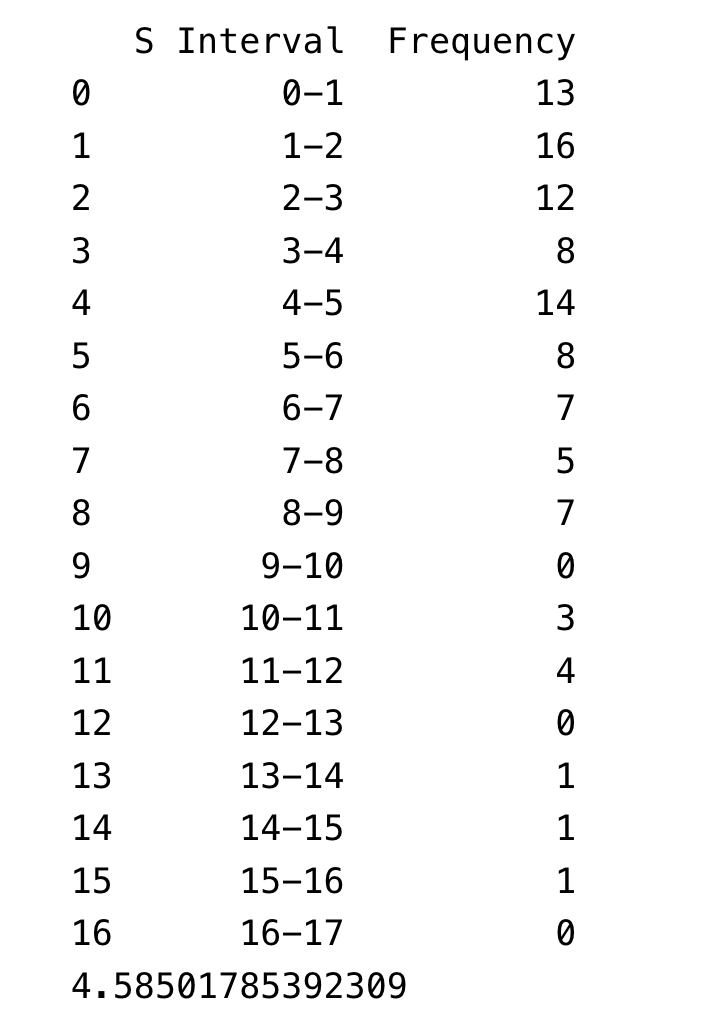
Where 𝐘ₜ and 𝐗ₜ were generated as independent random walks, each of length 50. The values 𝐒 = |𝛽̂₁| / √(𝐒𝐄̂(𝛽̂₁)), representing the statistic for testing the significance of 𝛽₁, for 100 simulations will be reported in the table below.

Table 1: Regressing two independent random walks

The null hypothesis of no relationship between 𝐘ₜ and 𝐗ₜ is rejected at the 5% level if 𝐒 > 2. This table shows that the null hypothesis (𝛽 = 0) is wrongly rejected in about a quarter (71 times) of all cases. This is awkward because the two variables are independent random walks, meaning there’s no actual relationship. Let’s break down why this happens.

If 𝛽̂₁ / 𝐒𝐄̂ follows a 𝐍(0,1), the expected value of 𝐒, its absolute value, should be √2 / π ≈ 0.8 (√2/π is the mean of the absolute value of a standard normal distribution). However, the simulation results show an average of 4.59, meaning the estimated 𝐒 is underestimated by a factor of:

4.59 / 0.8 = 5.7

In classical statistics, we usually use a t-test threshold of around 2 to check the significance of a coefficient. However, these results show that, in this case, you would need to use a threshold of 11.4 to properly test for significance:

2 × (4.59 / 0.8) = 11.4

Interpretation: We’ve just shown that including variables that don’t belong in the model — especially random walks — can lead to completely invalid significance tests for the coefficients.

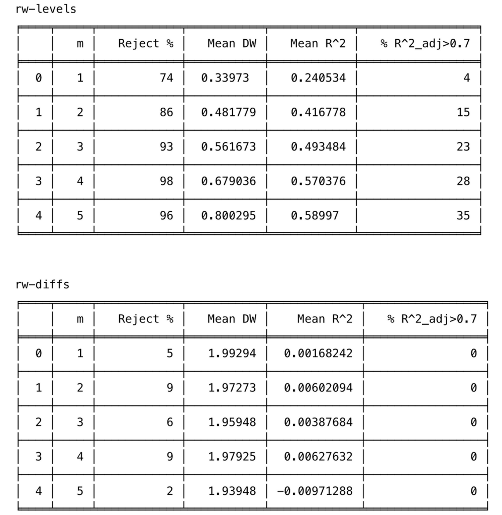
To make their simulations even clearer, Granger and Newbold (1974) ran a series of regressions using variables that follow either a random walk or an ARIMA(0,1,1) process.

Here is how they set up their simulations:

They regressed a dependent series 𝐘ₜ on m series 𝐗ⱼ,ₜ (with j = 1, 2, …, m), varying m from 1 to 5. The dependent series 𝐘ₜ and the independent series 𝐗ⱼ,ₜ follow the same types of processes, and they tested four cases:

  • Case 1 (Levels): 𝐘ₜ and 𝐗ⱼ,ₜ follow random walks.
  • Case 2 (Differences): They use the first differences of the random walks, which are stationary.
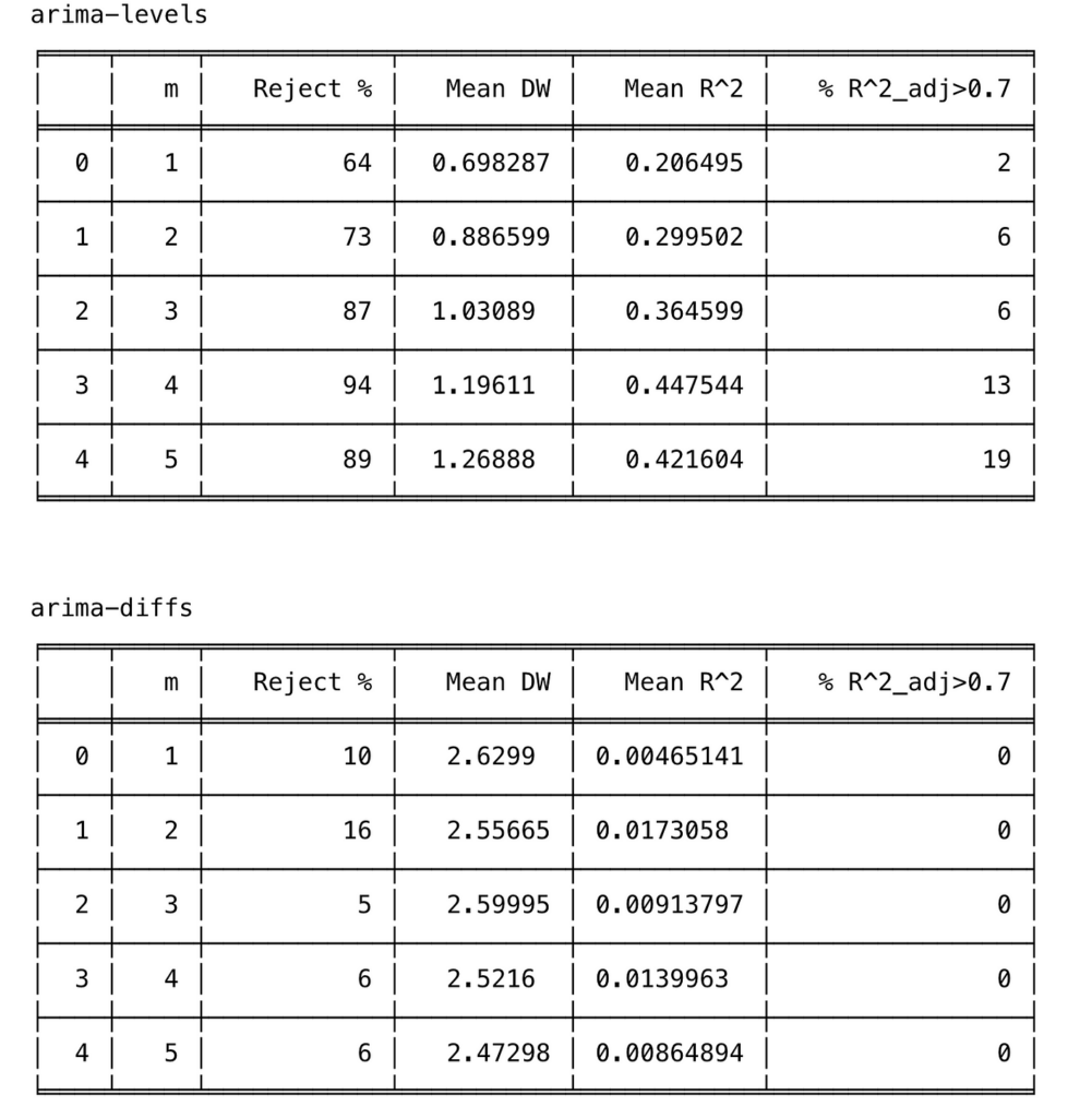
  • Case 3 (Levels): 𝐘ₜ and 𝐗ⱼ,ₜ follow ARIMA(0,1,1).
  • Case 4 (Differences): They use the first differences of the previous ARIMA(0,1,1) processes, which are stationary.

Each series has a length of 50 observations, and they ran 100 simulations for each case.

All error terms are distributed as 𝐍(0,1), and the ARIMA(0,1,1) series are derived as the sum of the random walk and independent white noise. The simulation results, based on 100 replications with series of length 50, are summarized in the next table.
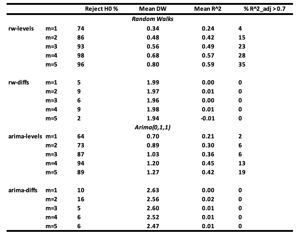
Table 2: Regressions of a series on m independent ‘explanatory’ series.

Interpretation of the results :

  • It is seen that the probability of not rejecting the null hypothesis of no relationship between 𝐘ₜ and 𝐗ⱼ,ₜ becomes very small when m ≥ 3 when regressions are made with random walk series (rw-levels). The 𝐑² and the mean Durbin-Watson increase. Similar results are obtained when the regressions are made with ARIMA(0,1,1) series (arima-levels).
  • When white noise series (rw-diffs) are used, classical regression analysis is valid since the error series will be white noise and least squares will be efficient.
  • However, when the regressions are made with the differences of ARIMA(0,1,1) series (arima-diffs) or first-order moving average series MA(1) process, the null hypothesis is rejected, on average:

(10 + 16 + 5 + 6 + 6) / 5 = 8.6

which is greater than 5% of the time.

If your variables are random walks or close to them, and you include unnecessary variables in your regression, you will often get fallacious results. High 𝐑² and low Durbin-Watson values do not confirm a true relationship but instead indicate a likely spurious one.

5. How to avoid spurious regression in time series

It’s really hard to come up with a complete list of ways to avoid spurious regressions. However, there are a few good practices you can follow to minimize the risk as much as possible.

If one performs a regression analysis with time series data and finds that the residuals are strongly autocorrelated, there is a serious problem when it comes to interpreting the coefficients of the equation. To check for autocorrelation in the residuals, one can use the Durbin-Watson test or the Portmanteau test.

Based on the study above, we can conclude that if a regression analysis performed with economical variables produces strongly autocorrelated residuals, meaning a low Durbin-Watson statistic, then the results of the analysis are likely to be spurious, whatever the value of the coefficient of determination R² observed.

In such cases, it is important to understand where the mis-specification comes from. According to the literature, misspecification usually falls into three categories : (i) the omission of a relevant variable, (ii) the inclusion of an irrelevant variable, or (iii) autocorrelation of the errors. Most of the time, mis-specification comes from a mix of these three sources.

To avoid spurious regression in a time series, several recommendations can be made:

  • The first recommendation is to select the right macroeconomic variables that are likely to explain the dependent variable. This can be done by reviewing the literature or consulting experts in the field.
  • The second recommendation is to stationarize the series by taking first differences. In most cases, the first differences of macroeconomic variables are stationary and still easy to interpret. For macroeconomic data, it’s strongly recommended to differentiate the series once to reduce the autocorrelation of the residuals, especially when the sample size is small. There is indeed sometimes strong serial correlation observed in these variables. A simple calculation shows that the first differences will almost always have much smaller serial correlations than the original series.
  • The third recommendation is to use the Box-Jenkins methodology to model each macroeconomic variable individually and then search for relationships between the series by relating the residuals from each individual model. The idea here is that the Box-Jenkins process extracts the explained part of the series, leaving the residuals, which contain only what can’t be explained by the series’ own past behavior. This makes it easier to check whether these unexplained parts (residuals) are related across variables.

6. Conclusion

Many econometrics textbooks warn about specification errors in regression models, but the problem still shows up in many published papers. Granger and Newbold (1974) highlighted the risk of spurious regressions, where you get a high paired with very low Durbin-Watson statistics.

Using Python simulations, we showed some of the main causes of these spurious regressions, especially including variables that don’t belong in the model and are highly autocorrelated. We also demonstrated how these issues can completely distort hypothesis tests on the coefficients.

Hopefully, this post will help reduce the risk of spurious regressions in future econometric analyses.

7. Appendice: Python code for simulation.

#####################################################Simulation Code for table 1 #####################################################

import numpy as np
import pandas as pd
import statsmodels.api as sm
import matplotlib.pyplot as plt

np.random.seed(123)
M = 100 
n = 50
S = np.zeros(M)
for i in range(M):
#---------------------------------------------------------------
# Generate the data
#---------------------------------------------------------------
    espilon_y = np.random.normal(0, 1, n)
    espilon_x = np.random.normal(0, 1, n)

    Y = np.cumsum(espilon_y)
    X = np.cumsum(espilon_x)
#---------------------------------------------------------------
# Fit the model
#---------------------------------------------------------------
    X = sm.add_constant(X)
    model = sm.OLS(Y, X).fit()
#---------------------------------------------------------------
# Compute the statistic
#------------------------------------------------------
    S[i] = np.abs(model.params[1])/model.bse[1]


#------------------------------------------------------ 
#              Maximum value of S
#------------------------------------------------------
S_max = int(np.ceil(max(S)))

#------------------------------------------------------ 
#                Create bins
#------------------------------------------------------
bins = np.arange(0, S_max + 2, 1)  

#------------------------------------------------------
#    Compute the histogram
#------------------------------------------------------
frequency, bin_edges = np.histogram(S, bins=bins)

#------------------------------------------------------
#    Create a dataframe
#------------------------------------------------------

df = pd.DataFrame({
    "S Interval": [f"{int(bin_edges[i])}-{int(bin_edges[i+1])}" for i in range(len(bin_edges)-1)],
    "Frequency": frequency
})
print(df)
print(np.mean(S))
#####################################################Simulation Code for table 2 #####################################################

import numpy as np
import pandas as pd
import statsmodels.api as sm
from statsmodels.stats.stattools import durbin_watson
from tabulate import tabulate

np.random.seed(1)  # Pour rendre les résultats reproductibles

#------------------------------------------------------
# Definition of functions
#------------------------------------------------------

def generate_random_walk(T):
    """
    Génère une série de longueur T suivant un random walk :
        Y_t = Y_{t-1} + e_t,
    où e_t ~ N(0,1).
    """
    e = np.random.normal(0, 1, size=T)
    return np.cumsum(e)

def generate_arima_0_1_1(T):
    """
    Génère un ARIMA(0,1,1) selon la méthode de Granger & Newbold :
    la série est obtenue en additionnant une marche aléatoire et un bruit blanc indépendant.
    """
    rw = generate_random_walk(T)
    wn = np.random.normal(0, 1, size=T)
    return rw + wn

def difference(series):
    """
    Calcule la différence première d'une série unidimensionnelle.
    Retourne une série de longueur T-1.
    """
    return np.diff(series)

#------------------------------------------------------
# Paramètres
#------------------------------------------------------

T = 50           # longueur de chaque série
n_sims = 100     # nombre de simulations Monte Carlo
alpha = 0.05     # seuil de significativité

#------------------------------------------------------
# Definition of function for simulation
#------------------------------------------------------

def run_simulation_case(case_name, m_values=[1,2,3,4,5]):
    """
    case_name : un identifiant pour le type de génération :
        - 'rw-levels' : random walk (levels)
        - 'rw-diffs'  : differences of RW (white noise)
        - 'arima-levels' : ARIMA(0,1,1) en niveaux
        - 'arima-diffs'  : différences d'un ARIMA(0,1,1) => MA(1)
    
    m_values : liste du nombre de régresseurs.
    
    Retourne un DataFrame avec pour chaque m :
        - % de rejets de H0
        - Durbin-Watson moyen
        - R^2_adj moyen
        - % de R^2 > 0.1
    """
    results = []
    
    for m in m_values:
        count_reject = 0
        dw_list = []
        r2_adjusted_list = []
        
        for _ in range(n_sims):
#--------------------------------------
# 1) Generation of independents de Y_t and X_{j,t}.
#----------------------------------------
            if case_name == 'rw-levels':
                Y = generate_random_walk(T)
                Xs = [generate_random_walk(T) for __ in range(m)]
            
            elif case_name == 'rw-diffs':
                # Y et X sont les différences d'un RW, i.e. ~ white noise
                Y_rw = generate_random_walk(T)
                Y = difference(Y_rw)
                Xs = []
                for __ in range(m):
                    X_rw = generate_random_walk(T)
                    Xs.append(difference(X_rw))
                # NB : maintenant Y et Xs ont longueur T-1
                # => ajuster T_effectif = T-1
                # => on prendra T_effectif points pour la régression
            
            elif case_name == 'arima-levels':
                Y = generate_arima_0_1_1(T)
                Xs = [generate_arima_0_1_1(T) for __ in range(m)]
            
            elif case_name == 'arima-diffs':
                # Différences d'un ARIMA(0,1,1) => MA(1)
                Y_arima = generate_arima_0_1_1(T)
                Y = difference(Y_arima)
                Xs = []
                for __ in range(m):
                    X_arima = generate_arima_0_1_1(T)
                    Xs.append(difference(X_arima))
            
            # 2) Prépare les données pour la régression
            #    Selon le cas, la longueur est T ou T-1
            if case_name in ['rw-levels','arima-levels']:
                Y_reg = Y
                X_reg = np.column_stack(Xs) if m>0 else np.array([])
            else:
                # dans les cas de différences, la longueur est T-1
                Y_reg = Y
                X_reg = np.column_stack(Xs) if m>0 else np.array([])
            
            # 3) Régression OLS
            X_with_const = sm.add_constant(X_reg)  # Ajout de l'ordonnée à l'origine
            model = sm.OLS(Y_reg, X_with_const).fit()
            
            # 4) Test global F : H0 : tous les beta_j = 0
            #    On regarde si p-value < alpha
            if model.f_pvalue is not None and model.f_pvalue  0.7)
        
        results.append({
            'm': m,
            'Reject %': reject_percent,
            'Mean DW': dw_mean,
            'Mean R^2': r2_mean,
            '% R^2_adj>0.7': r2_above_0_7_percent
        })
    
    return pd.DataFrame(results)
    
#------------------------------------------------------
# Application of the simulation
#------------------------------------------------------       

cases = ['rw-levels', 'rw-diffs', 'arima-levels', 'arima-diffs']
all_results = {}

for c in cases:
    df_res = run_simulation_case(c, m_values=[1,2,3,4,5])
    all_results[c] = df_res

#------------------------------------------------------
# Store data in table
#------------------------------------------------------

for case, df_res in all_results.items():
    print(f"nn{case}")
    print(tabulate(df_res, headers='keys', tablefmt='fancy_grid'))
References

  • Granger, Clive WJ, and Paul Newbold. 1974. “Spurious Regressions in Econometrics.” Journal of Econometrics 2 (2): 111–20.
  • Knowles, EAG. 1954. “Exercises in Theoretical Statistics.” Oxford University Press.
Shape
Shape
Stay Ahead

Explore More Insights

Stay ahead with more perspectives on cutting-edge power, infrastructure, energy,  bitcoin and AI solutions. Explore these articles to uncover strategies and insights shaping the future of industries.

Shape

Russian Crude Output Rose Last Month

Russia’s crude oil production edged up in October, but remained below its OPEC+ quota as international pressure mounted on the country’s energy sector. Russia pumped an average 9.411 million barrels a day last month, people with knowledge of the data said, asking not to be identified discussing confidential information. While that’s 43,000 barrels a day higher than in September, it’s 70,000 a day below a quota that includes compensation cuts for previous overproduction, Bloomberg calculations show. Oil watchers are closely following Russian production data to assess the impact of sanctions — and Ukrainian drone strikes — against the country’s energy industry. The latest US penalties on the sector, which hit oil giants Rosneft PJSC and Lukoil PJSC, have already eroded crude exports as some refiners in India, China and Turkey prove less willing to take sanctioned barrels. Meanwhile, Ukrainian attacks have intensified, putting pressure on Russia’s crude-processing sector even as refinery owners rush to repair infrastructure.  If Moscow eventually finds itself unable to find buyers for oil from its sanctioned producers, and struggles to restore refining, it’ll be forced to halt output at some fields, risking damage to wells. The Energy Ministry didn’t immediately respond to a request for comment on the production data. Deputy Prime Minister Alexander Novak said last month that the nation has capacity to raise oil production further, but will do it gradually, according to Tass news service. Compensation Cuts Russia, historically one of the biggest laggards in complying with OPEC+ output agreements, has agreed to make additional cuts to compensate for previous overproduction. The monthly schedule for those curbs has been regularly revised, with the latest plan published earlier this month.  It shows that October was the last month when Russia had to make such cuts. Moscow’s pledge to reduce daily output by 10,000 barrels below a quota of 9.491

Read More »

Oil Rises but Logs Second Weekly Loss

Oil rose on Friday but still notched a second weekly loss as the market continued to weigh the threat to output from sanctions on Russia against a looming oversupply. West Texas Intermediate futures rose around 0.5% to settle below $60 a barrel, but were still down for the week. Adding to fears of a glut, oil prices have also been buffeted by swings in equity markets this week. Meanwhile, the White House’s move to clamp down on the buying of Russian crude led oil trading giant Gunvor Group to withdraw an offer for the international assets of Lukoil PJSC. The fate of the assets, which include stakes in oil fields, refineries and gas stations, remains unclear. One possible exception to that crackdown could emerge soon: President Donald Trump signaled an openness to exempting Hungary from sanctions on Russian energy purchases as he hosted Prime Minister Viktor Orban, briefly pushing futures to intraday lows. The development appeared to allay shortage fears, given that Budapest imports over 90% of its crude from Moscow. Senior industry figures have warned the latest US curbs on Russia’s two largest oil companies are beginning to have an impact on the market, particularly in diesel, where prices have been surging in recent days, with time spreads for the fuel signaling supply pressure. At the same time, the US measures have come against a backdrop of oversupply that has weighed on key crude oil metrics. The spread between the nearest West Texas Intermediate futures closed at the weakest level since February on Thursday. “If the market flips to contango, we may see more bearish funds enter the crude space,” said Dennis Kissler, senior vice president for trading at BOK Financial said of the potential that longer-dated contracts trade at a premium to nearer-term ones. “Most traders remain surprised

Read More »

Gunvor Scraps Lukoil Deal

Commodity trader Gunvor Group has withdrawn its offer for the international assets of sanctioned Russian oil producer Lukoil PJSC after the US Treasury Department called it “the Kremlin’s puppet” and said the oil and gas trader would never get a license. Gunvor pushed back on the Treasury comment on social media, calling it “fundamentally misinformed and false.” The Geneva-based company said it would seek to correct a “clear misunderstanding” but that it would withdraw its bid for now. President Trump has been clear that the war must end immediately. As long as Putin continues the senseless killings, the Kremlin’s puppet, Gunvor, will never get a license to operate and profit. — Treasury Department (@USTreasury) November 6, 2025 The comment is a remarkable volte-face after a week in which Gunvor has been in talks with the US Office of Foreign Assets Control, part of the Treasury Department, and other bodies in charge of sanctions to help press its case for a deal that would have transformed it into an integrated oil producing and processing colossus. Gunvor swooped on the assets at the end of last month following the US blacklisting of Lukoil and fellow Russian oil giant Rosneft PJSC, and its exit may leave the door open to other suitors. Gunvor on Thursday also announced it had raised $2.81 billion in a credit facility financed by US arms of global banks. Like other major commodity traders, the firm funds the bulk of its trades of oil, gas and metals around the world with bank financing. For the trader, the comments are likely to revive questions about its connections in Moscow at a time when many oil industry participants are wary of any links to Russia.  The trader’s co-founder, Gennady Timchenko, is a friend of Russian President Vladimir Putin, and when the US imposed sanctions

Read More »

Ship With Russia Oil Makes Rare Move Offshore India

A tanker carrying crude from recently-sanctioned Rosneft PJSC has made a rare cargo transfer off Mumbai, as the Trump administration ramps up its scrutiny of India’s oil trade with Russia. But the unusual move has puzzled traders. The cargo was transferred from one blacklisted tanker to another sanctioned ship, meaning there’s been no attempt to hide its origin — typical of such a move — and the crude is still heading for an Indian port: Kochi in the south, rather than Mumbai on the west coast. India’s purchases of Russian oil have drawn the ire of President Donald Trump, and the US penalties on Rosneft along with Lukoil PJSC are expected to severely impact the trade. The market is keenly watching for disruptions to established flows before a grace period related to the sanctions ends later this month. “What we’re seeing now is this uncertainty in the market about what the sanctions risks are,” said Rachel Ziemba, an analyst at the Center for a New American Security in Washington. “The net result is more ship-to-ship transfers, more subterfuge, longer routes, more complicated transactions.” The Fortis took around 720,000 barrels of Russian Urals from Ailana on Tuesday near Mumbai, according to ship-tracking data compiled by Bloomberg, Kpler and Vortexa. The cargo was collected from the Baltic port of Ust-Luga before the US sanctioned Rosneft, and Ailana had idled in the area for nearly two weeks with no clear reason.  Ailana is on its way back to Russia, while Fortis is expected to arrive at Kochi early next week with the cargo, ship-tracking data shows. Both vessels have been sanctioned by the European Union and the UK. Fortis’ owner and manager — Vietnam-based Pacific Logistic & Maritime and North Star Ship Management — didn’t respond to emailed requests for comment. There are no contact details on maritime database

Read More »

Petrobras Ramps Up Production at Major Oilfield

Brazil’s state oil producer Petrobras is accelerating production from the world’s biggest deep-water field, helping the company raise dividends even as crude prices hover near a five-year low and the global market braces for glut. Petroleo Brasileiro SA’s output from the Buzios field off the coast of Rio de Janeiro reached one million barrels a day last month after the sixth floating production vessel at the site reached its capacity three months ahead of schedule. The company reported it would pay $2.3 billion in dividends on Thursday, slightly above expectations and more than the previous quarter.  The field, part of the pre-salt basin that 18 years ago made Brazil one of the world’s oil hottest oil regions, is now Petrobras’ last big growth engine. Its rapid development has allowed the nation to increase production more than any other non-OPEC country apart from the US in the past year and provided Petrobras with a crucial source of revenue as it hunts for the next big discovery.  The flood of crude from Buzios comes as global oil futures have slipped 15 percent this year as OPEC and its allies have ramped up production, fueling concerns the market will soon be awash in crude. The chief executive officer of Mercuria, the commodities giant, said at a conference in Abu Dhabi Wednesday that an oversupply is likely to be as much as 2 million barrels a day next year. The company’s record exports helped it increase its net income to $6 billion from the previous quarter despite low prices, it said in its earnings release on Thursday.  At the Buzios field, the Almirante Tamandare floating production and storage vessel reached production of 225,000 barrels a day ahead of schedule in August, helping to bring exports to a record. Last week, it reached 270,000 barrels a

Read More »

Southwest Power Pool to develop 765-kV regional transmission ‘backbone’

Listen to the article 4 min This audio is auto-generated. Please let us know if you have feedback. Dive Brief: The Southwest Power Pool board of directors on Wednesday approved an $8.6 billion slate of 50 transmission projects across its 14-state footprint. The projects are intended to help the grid operator meet peak demand, which it expects will double, to reach 109 GW, in the next 10 years. Key to the 2025 Integrated Transmission Plan is development of a 765-kV regional transmission “backbone” that can carry four times the power SPP’s existing 345-kV lines do, and do so more efficiently. The grid operator’s transmission system “is at capacity and forecasted load growth will only exacerbate the existing strain,” it said. “Simply adding new generation will not resolve the challenges.” 765-kV transmission lines are the highest operating voltages in the U.S. but are new in both SPP and in the neighboring Electric Reliability Council of Texas market. Texas regulators approved the higher voltage lines for the first time in April. Dive Insight: Transmission developers in SPP and ERCOT are turning to 765-kV projects to mitigate line losses and move greater volumes of power into demand centers at a time when electricity demand is expected to rise significantly. “With the new load being integrated into the system, SPP could see an increase in the footprint’s annual energy consumption by as much as 136%,” the grid operator said in its ITP. “Investments in transmission are the key to keep costs low, maintain reliability, and power economic growth.” Even under conservative assumptions, SPP forecasts a 35% increase in demand, “making timely transmission investment essential,” the grid operator said. SPP selected Xcel Energy in February to construct the first 765-kV lines in its footprint. Those lines were identified in its 2024 plan. AEP Texas will build

Read More »

Designing the AI Century: 7×24 Exchange Fall ’25 Charts the New Data Center Industrial Stack

SMRs and the AI Power Gap: Steve Fairfax Separates Promise from Physics If NVIDIA’s Sean Young made the case for AI factories, Steve Fairfax offered a sobering counterweight: even the smartest factories can’t run without power—and not just any power, but constant, high-availability, clean generation at a scale utilities are increasingly struggling to deliver. In his keynote “Small Modular Reactors for Data Centers,” Fairfax, president of Oresme and one of the data center industry’s most seasoned voices on reliability, walked through the long arc from nuclear fusion research to today’s resurgent interest in fission at modular scale. His presentation blended nuclear engineering history with pragmatic counsel for AI-era infrastructure leaders: SMRs are promising, but their road to reality is paved with physics, fuel, and policy—not PowerPoint. From Fusion Research to Data Center Reliability Fairfax began with his own story—a career that bridges nuclear reliability and data center engineering. As a young physicist and electrical engineer at MIT, he helped build the Alcator C-MOD fusion reactor, a 400-megawatt research facility that heated plasma to 100 million degrees with 3 million amps of current. The magnet system alone drew 265,000 amps at 1,400 volts, producing forces measured in millions of pounds. It was an extreme experiment in controlled power, and one that shaped his later philosophy: design for failure, test for truth, and assume nothing lasts forever. When the U.S. cooled on fusion power in the 1990s, Fairfax applied nuclear reliability methods to data center systems—quantifying uptime and redundancy with the same math used for reactor safety. By 1994, he was consulting for hyperscale pioneers still calling 10 MW “monstrous.” Today’s 400 MW campuses, he noted, are beginning to look a lot more like reactors in their energy intensity—and increasingly, in their regulatory scrutiny. Defining the Small Modular Reactor Fairfax defined SMRs

Read More »

Top network and data center events 2025 & 2026

Denise Dubie is a senior editor at Network World with nearly 30 years of experience writing about the tech industry. Her coverage areas include AIOps, cybersecurity, networking careers, network management, observability, SASE, SD-WAN, and how AI transforms enterprise IT. A seasoned journalist and content creator, Denise writes breaking news and in-depth features, and she delivers practical advice for IT professionals while making complex technology accessible to all. Before returning to journalism, she held senior content marketing roles at CA Technologies, Berkshire Grey, and Cisco. Denise is a trusted voice in the world of enterprise IT and networking.

Read More »

Google’s cheaper, faster TPUs are here, while users of other AI processors face a supply crunch

Opportunities for the AI industry LLM vendors such as OpenAI and Anthropic, which still have relatively young code bases and are continuously evolving them, also have much to gain from the arrival of Ironwood for training their models, said Forrester vice president and principal analyst Charlie Dai. In fact, Anthropic has already agreed to procure 1 million TPUs for training and its models and using them for inferencing. Other, smaller vendors using Google’s TPUs for training models include Lightricks and Essential AI. Google has seen a steady increase in demand for its TPUs (which it also uses to run interna services), and is expected to buy $9.8 billion worth of TPUs from Broadcom this year, compared to $6.2 billion and $2.04 billion in 2024 and 2023 respectively, according to Harrowell. “This makes them the second-biggest AI chip program for cloud and enterprise data centers, just tailing Nvidia, with approximately 5% of the market. Nvidia owns about 78% of the market,” Harrowell said. The legacy problem While some analysts were optimistic about the prospects for TPUs in the enterprise, IDC research director Brandon Hoff said enterprises will most likely to stay away from Ironwood or TPUs in general because of their existing code base written for other platforms. “For enterprise customers who are writing their own inferencing, they will be tied into Nvidia’s software platform,” Hoff said, referring to CUDA, the software platform that runs on Nvidia GPUs. CUDA was released to the public in 2007, while the first version of TensorFlow has only been around since 2015.

Read More »

Cisco launches AI infrastructure, AI practitioner certifications

“This new certification focuses on artificial intelligence and machine learning workloads, helping technical professionals become AI-ready and successfully embed AI into their workflows,” said Pat Merat, vice president at Learn with Cisco, in a blog detailing the new AI Infrastructure Specialist certification. “The certification validates a candidate’s comprehensive knowledge in designing, implementing, operating, and troubleshooting AI solutions across Cisco infrastructure.” Separately, the AITECH certification is part of the Cisco AI Infrastructure track, which complements its existing networking, data center, and security certifications. Cisco says the AITECH cert training is intended for network engineers, system administrators, solution architects, and other IT professionals who want to learn how AI impacts enterprise infrastructure. The training curriculum covers topics such as: Utilizing AI for code generation, refactoring, and using modern AI-assisted coding workflows. Using generative AI for exploratory data analysis, data cleaning, transformation, and generating actionable insights. Designing and implementing multi-step AI-assisted workflows and understanding complex agentic systems for automation. Learning AI-powered requirements, evaluating customization approaches, considering deployment strategies, and designing robust AI workflows. Evaluating, fine-tuning, and deploying pre-trained AI models, and implementing Retrieval Augmented Generation (RAG) systems. Monitoring, maintaining, and optimizing AI-powered workflows, ensuring data integrity and security. AITECH certification candidates will learn how to use AI to enhance productivity, automate routine tasks, and support the development of new applications. The training program includes hands-on labs and simulations to demonstrate practical use cases for AI within Cisco and multi-vendor environments.

Read More »

Chip-to-Grid Gets Bought: Eaton, Vertiv, and Daikin Deals Imply a New Thermal Capital Cycle

This week delivered three telling acquisitions that mark a turning point for the global data center supply chain; and more specifically, for the high-density liquid cooling mega-play now unfolding across the power-thermal continuum. Eaton is acquiring Boyd Thermal for $9.5 billion from Goldman Sachs Asset Management. Vertiv is buying PurgeRite for about $1 billion from Milton Street Capital. And Daikin Applied has moved to acquire Chilldyne, one of the most proven negative-pressure direct-to-chip pioneers. On paper, they’re three distinct transactions. In reality, they’re chapters in the same story: the acceleration of strategic vertical integration around thermal infrastructure for AI-class compute. The Equity Layer: Private Capital Builds, Strategics Buy From an equity standpoint, these are classic handoff moments between private-equity construction and corporate consolidation. Goldman Sachs built Boyd Thermal into a global platform spanning cold plates, CDUs, and high-density liquid loop design, now sold to Eaton at an enterprise multiple north of 5× 2026E revenue. Milton Street Capital took PurgeRite from a specialist contractor in fluid flushing and commissioning into a nationwide services platform. And Daikin, long synonymous with chillers and air-side thermal, is crossing the liquid Rubicon by buying its way into the D2C ecosystem. Each deal crystallizes a simple fact: liquid cooling is no longer an adjunct; it’s core infrastructure. Private equity did its job scaling the parts. Strategic players are now paying up for the system. Eaton’s Bid: The Chip-to-Grid Thesis For Eaton, Boyd Thermal is the final missing piece in its “chip-to-grid” thesis. The company already owns the electrical side of the data center: UPS, busway, switchgear, and monitoring. Boyd plugs the thermal gap, allowing Eaton to market full rack-to-substation solutions for AI loads in the 50–100 kW+ range. It’s a statement acquisition that places Eaton squarely against Schneider Electric, Vertiv and ABB in the race to

Read More »

Space: The final frontier for data processing

There are, however, a couple of reasons why data centers in space are being considered. There are plenty of reports about how the increased amount of AI processing is affecting power consumption within data centers; the World Economic Forum has estimated that the power required to handle AI is increasing at a rate of between 26% and 36% annually. Therefore, it is not surprising that organizations are looking at other options. But an even more pressing reason for orbiting data centers is to handle the amount of data that is being produced by existing satellites, Judge said. “Essentially, satellites are gathering a lot more data than can be sent to earth, because downlinks are a bottleneck,” he noted. “With AI capacity in orbit, they could potentially analyze more of this data, extract more useful information, and send insights back to earth. My overall feeling is that any more data processing in space is going to be driven by space processing needs.” And China may already be ahead of the game. Last year, Guoxing Aerospace  launched 12 satellites, forming a space-based computing network dubbed the Three-Body Computing Constellation. When completed, it will contain 2,800 satellites, all handling the orchestration and processing of data, taking edge computing to a new dimension.

Read More »

Microsoft will invest $80B in AI data centers in fiscal 2025

And Microsoft isn’t the only one that is ramping up its investments into AI-enabled data centers. Rival cloud service providers are all investing in either upgrading or opening new data centers to capture a larger chunk of business from developers and users of large language models (LLMs).  In a report published in October 2024, Bloomberg Intelligence estimated that demand for generative AI would push Microsoft, AWS, Google, Oracle, Meta, and Apple would between them devote $200 billion to capex in 2025, up from $110 billion in 2023. Microsoft is one of the biggest spenders, followed closely by Google and AWS, Bloomberg Intelligence said. Its estimate of Microsoft’s capital spending on AI, at $62.4 billion for calendar 2025, is lower than Smith’s claim that the company will invest $80 billion in the fiscal year to June 30, 2025. Both figures, though, are way higher than Microsoft’s 2020 capital expenditure of “just” $17.6 billion. The majority of the increased spending is tied to cloud services and the expansion of AI infrastructure needed to provide compute capacity for OpenAI workloads. Separately, last October Amazon CEO Andy Jassy said his company planned total capex spend of $75 billion in 2024 and even more in 2025, with much of it going to AWS, its cloud computing division.

Read More »

John Deere unveils more autonomous farm machines to address skill labor shortage

Join our daily and weekly newsletters for the latest updates and exclusive content on industry-leading AI coverage. Learn More Self-driving tractors might be the path to self-driving cars. John Deere has revealed a new line of autonomous machines and tech across agriculture, construction and commercial landscaping. The Moline, Illinois-based John Deere has been in business for 187 years, yet it’s been a regular as a non-tech company showing off technology at the big tech trade show in Las Vegas and is back at CES 2025 with more autonomous tractors and other vehicles. This is not something we usually cover, but John Deere has a lot of data that is interesting in the big picture of tech. The message from the company is that there aren’t enough skilled farm laborers to do the work that its customers need. It’s been a challenge for most of the last two decades, said Jahmy Hindman, CTO at John Deere, in a briefing. Much of the tech will come this fall and after that. He noted that the average farmer in the U.S. is over 58 and works 12 to 18 hours a day to grow food for us. And he said the American Farm Bureau Federation estimates there are roughly 2.4 million farm jobs that need to be filled annually; and the agricultural work force continues to shrink. (This is my hint to the anti-immigration crowd). John Deere’s autonomous 9RX Tractor. Farmers can oversee it using an app. While each of these industries experiences their own set of challenges, a commonality across all is skilled labor availability. In construction, about 80% percent of contractors struggle to find skilled labor. And in commercial landscaping, 86% of landscaping business owners can’t find labor to fill open positions, he said. “They have to figure out how to do

Read More »

2025 playbook for enterprise AI success, from agents to evals

Join our daily and weekly newsletters for the latest updates and exclusive content on industry-leading AI coverage. Learn More 2025 is poised to be a pivotal year for enterprise AI. The past year has seen rapid innovation, and this year will see the same. This has made it more critical than ever to revisit your AI strategy to stay competitive and create value for your customers. From scaling AI agents to optimizing costs, here are the five critical areas enterprises should prioritize for their AI strategy this year. 1. Agents: the next generation of automation AI agents are no longer theoretical. In 2025, they’re indispensable tools for enterprises looking to streamline operations and enhance customer interactions. Unlike traditional software, agents powered by large language models (LLMs) can make nuanced decisions, navigate complex multi-step tasks, and integrate seamlessly with tools and APIs. At the start of 2024, agents were not ready for prime time, making frustrating mistakes like hallucinating URLs. They started getting better as frontier large language models themselves improved. “Let me put it this way,” said Sam Witteveen, cofounder of Red Dragon, a company that develops agents for companies, and that recently reviewed the 48 agents it built last year. “Interestingly, the ones that we built at the start of the year, a lot of those worked way better at the end of the year just because the models got better.” Witteveen shared this in the video podcast we filmed to discuss these five big trends in detail. Models are getting better and hallucinating less, and they’re also being trained to do agentic tasks. Another feature that the model providers are researching is a way to use the LLM as a judge, and as models get cheaper (something we’ll cover below), companies can use three or more models to

Read More »

OpenAI’s red teaming innovations define new essentials for security leaders in the AI era

Join our daily and weekly newsletters for the latest updates and exclusive content on industry-leading AI coverage. Learn More OpenAI has taken a more aggressive approach to red teaming than its AI competitors, demonstrating its security teams’ advanced capabilities in two areas: multi-step reinforcement and external red teaming. OpenAI recently released two papers that set a new competitive standard for improving the quality, reliability and safety of AI models in these two techniques and more. The first paper, “OpenAI’s Approach to External Red Teaming for AI Models and Systems,” reports that specialized teams outside the company have proven effective in uncovering vulnerabilities that might otherwise have made it into a released model because in-house testing techniques may have missed them. In the second paper, “Diverse and Effective Red Teaming with Auto-Generated Rewards and Multi-Step Reinforcement Learning,” OpenAI introduces an automated framework that relies on iterative reinforcement learning to generate a broad spectrum of novel, wide-ranging attacks. Going all-in on red teaming pays practical, competitive dividends It’s encouraging to see competitive intensity in red teaming growing among AI companies. When Anthropic released its AI red team guidelines in June of last year, it joined AI providers including Google, Microsoft, Nvidia, OpenAI, and even the U.S.’s National Institute of Standards and Technology (NIST), which all had released red teaming frameworks. Investing heavily in red teaming yields tangible benefits for security leaders in any organization. OpenAI’s paper on external red teaming provides a detailed analysis of how the company strives to create specialized external teams that include cybersecurity and subject matter experts. The goal is to see if knowledgeable external teams can defeat models’ security perimeters and find gaps in their security, biases and controls that prompt-based testing couldn’t find. What makes OpenAI’s recent papers noteworthy is how well they define using human-in-the-middle

Read More »