Stay Ahead, Stay ONMINE

R.E.D.: Scaling Text Classification with Expert Delegation

With the new age of problem-solving augmented by Large Language Models (LLMs), only a handful of problems remain that have subpar solutions. Most classification problems (at a PoC level) can be solved by leveraging LLMs at 70–90% Precision/F1 with just good prompt engineering techniques, as well as adaptive in-context-learning (ICL) examples. What happens when you want to consistently achieve performance higher than that — when prompt engineering no longer suffices? The classification conundrum Text classification is one of the oldest and most well-understood examples of supervised learning. Given this premise, it should really not be hard to build robust, well-performing classifiers that handle a large number of input classes, right…? Welp. It is. It actually has to do a lot more with the ‘constraints’ that the algorithm is generally expected to work under: low amount of training data per class high classification accuracy (that plummets as you add more classes) possible addition of new classes to an existing subset of classes quick training/inference cost-effectiveness (potentially) really large number of training classes (potentially) endless required retraining of some classes due to data drift, etc. Ever tried building a classifier beyond a few dozen classes under these conditions? (I mean, even GPT could probably do a great job up to ~30 text classes with just a few samples…) Considering you take the GPT route — If you have more than a couple dozen classes or a sizeable amount of data to be classified, you are gonna have to reach deep into your pockets with the system prompt, user prompt, few shot example tokens that you will need to classify one sample. That is after making peace with the throughput of the API, even if you are running async queries. In applied ML, problems like these are generally tricky to solve since they don’t fully satisfy the requirements of supervised learning or aren’t cheap/fast enough to be run via an LLM. This particular pain point is what the R.E.D algorithm addresses: semi-supervised learning, when the training data per class is not enough to build (quasi)traditional classifiers. The R.E.D. algorithm R.E.D: Recursive Expert Delegation is a novel framework that changes how we approach text classification. This is an applied ML paradigm — i.e., there is no fundamentally different architecture to what exists, but its a highlight reel of ideas that work best to build something that is practical and scalable. In this post, we will be working through a specific example where we have a large number of text classes (100–1000), each class only has few samples (30–100), and there are a non-trivial number of samples to classify (10,000–100,000). We approach this as a semi-supervised learning problem via R.E.D. Let’s dive in. How it works simple representation of what R.E.D. does Instead of having a single classifier classify between a large number of classes, R.E.D. intelligently: Divides and conquers — Break the label space (large number of input labels) into multiple subsets of labels. This is a greedy label subset formation approach. Learns efficiently — Trains specialized classifiers for each subset. This step focuses on building a classifier that oversamples on noise, where noise is intelligently modeled as data from other subsets. Delegates to an expert — Employes LLMs as expert oracles for specific label validation and correction only, similar to having a team of domain experts. Using an LLM as a proxy, it empirically ‘mimics’ how a human expert validates an output. Recursive retraining — Continuously retrains with fresh samples added back from the expert until there are no more samples to be added/a saturation from information gain is achieved The intuition behind it is not very hard to grasp: Active Learning employs humans as domain experts to consistently ‘correct’ or ‘validate’ the outputs from an ML model, with continuous training. This stops when the model achieves acceptable performance. We intuit and rebrand the same, with a few clever innovations that will be detailed in a research pre-print later. Let’s take a deeper look… Greedy subset selection with least similar elements When the number of input labels (classes) is high, the complexity of learning a linear decision boundary between classes increases. As such, the quality of the classifier deteriorates as the number of classes increases. This is especially true when the classifier does not have enough samples to learn from — i.e. each of the training classes has only a few samples. This is very reflective of a real-world scenario, and the primary motivation behind the creation of R.E.D. Some ways of improving a classifier’s performance under these constraints: Restrict the number of classes a classifier needs to classify between Make the decision boundary between classes clearer, i.e., train the classifier on highly dissimilar classes Greedy Subset Selection does exactly this — since the scope of the problem is Text Classification, we form embeddings of the training labels, reduce their dimensionality via UMAP, then form S subsets from them. Each of the S subsets has elements as n training labels. We pick training labels greedily, ensuring that every label we pick for the subset is the most dissimilar label w.r.t. the other labels that exist in the subset: import numpy as np from sklearn.metrics.pairwise import cosine_similarity def avg_embedding(candidate_embeddings): return np.mean(candidate_embeddings, axis=0) def get_least_similar_embedding(target_embedding, candidate_embeddings): similarities = cosine_similarity(target_embedding, candidate_embeddings) least_similar_index = np.argmin(similarities) # Use argmin to find the index of the minimum least_similar_element = candidate_embeddings[least_similar_index] return least_similar_element def get_embedding_class(embedding, embedding_map): reverse_embedding_map = {value: key for key, value in embedding_map.items()} return reverse_embedding_map.get(embedding) # Use .get() to handle missing keys gracefully def select_subsets(embeddings, n): visited = {cls: False for cls in embeddings.keys()} subsets = [] current_subset = [] while any(not visited[cls] for cls in visited): for cls, average_embedding in embeddings.items(): if not current_subset: current_subset.append(average_embedding) visited[cls] = True elif len(current_subset) >= n: subsets.append(current_subset.copy()) current_subset = [] else: subset_average = avg_embedding(current_subset) remaining_embeddings = [emb for cls_, emb in embeddings.items() if not visited[cls_]] if not remaining_embeddings: break # handle edge case least_similar = get_least_similar_embedding(target_embedding=subset_average, candidate_embeddings=remaining_embeddings) visited_class = get_embedding_class(least_similar, embeddings) if visited_class is not None: visited[visited_class] = True current_subset.append(least_similar) if current_subset: # Add any remaining elements in current_subset subsets.append(current_subset) return subsets the result of this greedy subset sampling is all the training labels clearly boxed into subsets, where each subset has at most only n classes. This inherently makes the job of a classifier easier, compared to the original S classes it would have to classify between otherwise! Semi-supervised classification with noise oversampling Cascade this after the initial label subset formation — i.e., this classifier is only classifying between a given subset of classes. Picture this: when you have low amounts of training data, you absolutely cannot create a hold-out set that is meaningful for evaluation. Should you do it at all? How do you know if your classifier is working well? We approached this problem slightly differently — we defined the fundamental job of a semi-supervised classifier to be pre-emptive classification of a sample. This means that regardless of what a sample gets classified as it will be ‘verified’ and ‘corrected’ at a later stage: this classifier only needs to identify what needs to be verified. As such, we created a design for how it would treat its data: n+1 classes, where the last class is noise noise: data from classes that are NOT in the current classifier’s purview. The noise class is oversampled to be 2x the average size of the data for the classifier’s labels Oversampling on noise is a faux-safety measure, to ensure that adjacent data that belongs to another class is most likely predicted as noise instead of slipping through for verification. How do you check if this classifier is working well — in our experiments, we define this as the number of ‘uncertain’ samples in a classifier’s prediction. Using uncertainty sampling and information gain principles, we were effectively able to gauge if a classifier is ‘learning’ or not, which acts as a pointer towards classification performance. This classifier is consistently retrained unless there is an inflection point in the number of uncertain samples predicted, or there is only a delta of information being added iteratively by new samples. Proxy active learning via an LLM agent This is the heart of the approach — using an LLM as a proxy for a human validator. The human validator approach we are talking about is Active Labelling Let’s get an intuitive understanding of Active Labelling: Use an ML model to learn on a sample input dataset, predict on a large set of datapoints For the predictions given on the datapoints, a subject-matter expert (SME) evaluates ‘validity’ of predictions Recursively, new ‘corrected’ samples are added as training data to the ML model The ML model consistently learns/retrains, and makes predictions until the SME is satisfied by the quality of predictions For Active Labelling to work, there are expectations involved for an SME: when we expect a human expert to ‘validate’ an output sample, the expert understands what the task is a human expert will use judgement to evaluate ‘what else’ definitely belongs to a label L when deciding if a new sample should belong to L Given these expectations and intuitions, we can ‘mimic’ these using an LLM: give the LLM an ‘understanding’ of what each label means. This can be done by using a larger model to critically evaluate the relationship between {label: data mapped to label} for all labels. In our experiments, this was done using a 32B variant of DeepSeek that was self-hosted. Giving an LLM the capability to understand ‘why, what, and how’ Instead of predicting what is the correct label, leverage the LLM to identify if a prediction is ‘valid’ or ‘invalid’ only (i.e., LLM only has to answer a binary query). Reinforce the idea of what other valid samples for the label look like, i.e., for every pre-emptively predicted label for a sample, dynamically source c closest samples in its training (guaranteed valid) set when prompting for validation. The result? A cost-effective framework that relies on a fast, cheap classifier to make pre-emptive classifications, and an LLM that verifies these using (meaning of the label + dynamically sourced training samples that are similar to the current classification): import math def calculate_uncertainty(clf, sample): predicted_probabilities = clf.predict_proba(sample.reshape(1, -1))[0] # Reshape sample for predict_proba uncertainty = -sum(p * math.log(p, 2) for p in predicted_probabilities) return uncertainty def select_informative_samples(clf, data, k): informative_samples = [] uncertainties = [calculate_uncertainty(clf, sample) for sample in data] # Sort data by descending order of uncertainty sorted_data = sorted(zip(data, uncertainties), key=lambda x: x[1], reverse=True) # Get top k samples with highest uncertainty for sample, uncertainty in sorted_data[:k]: informative_samples.append(sample) return informative_samples def proxy_label(clf, llm_judge, k, testing_data): #llm_judge – any LLM with a system prompt tuned for verifying if a sample belongs to a class. Expected output is a bool : True or False. True verifies the original classification, False refutes it predicted_classes = clf.predict(testing_data) # Select k most informative samples using uncertainty sampling informative_samples = select_informative_samples(clf, testing_data, k) # List to store correct samples voted_data = [] # Evaluate informative samples with the LLM judge for sample in informative_samples: sample_index = testing_data.tolist().index(sample.tolist()) # changed from testing_data.index(sample) because of numpy array type issue predicted_class = predicted_classes[sample_index] # Check if LLM judge agrees with the prediction if llm_judge(sample, predicted_class): # If correct, add the sample to voted data voted_data.append(sample) # Return the list of correct samples with proxy labels return voted_data By feeding the valid samples (voted_data) to our classifier under controlled parameters, we achieve the ‘recursive’ part of our algorithm: Recursive Expert Delegation: R.E.D. By doing this, we were able to achieve close-to-human-expert validation numbers on controlled multi-class datasets. Experimentally, R.E.D. scales up to 1,000 classes while maintaining a competent degree of accuracy almost on par with human experts (90%+ agreement). I believe this is a significant achievement in applied ML, and has real-world uses for production-grade expectations of cost, speed, scale, and adaptability. The technical report, publishing later this year, highlights relevant code samples as well as experimental setups used to achieve given results. All images, unless otherwise noted, are by the author Interested in more details? Reach out to me over Medium or email for a chat!

With the new age of problem-solving augmented by Large Language Models (LLMs), only a handful of problems remain that have subpar solutions. Most classification problems (at a PoC level) can be solved by leveraging LLMs at 70–90% Precision/F1 with just good prompt engineering techniques, as well as adaptive in-context-learning (ICL) examples.

What happens when you want to consistently achieve performance higher than that — when prompt engineering no longer suffices?

The classification conundrum

Text classification is one of the oldest and most well-understood examples of supervised learning. Given this premise, it should really not be hard to build robust, well-performing classifiers that handle a large number of input classes, right…?

Welp. It is.

It actually has to do a lot more with the ‘constraints’ that the algorithm is generally expected to work under:

  • low amount of training data per class
  • high classification accuracy (that plummets as you add more classes)
  • possible addition of new classes to an existing subset of classes
  • quick training/inference
  • cost-effectiveness
  • (potentially) really large number of training classes
  • (potentially) endless required retraining of some classes due to data drift, etc.

Ever tried building a classifier beyond a few dozen classes under these conditions? (I mean, even GPT could probably do a great job up to ~30 text classes with just a few samples…)

Considering you take the GPT route — If you have more than a couple dozen classes or a sizeable amount of data to be classified, you are gonna have to reach deep into your pockets with the system prompt, user prompt, few shot example tokens that you will need to classify one sample. That is after making peace with the throughput of the API, even if you are running async queries.

In applied ML, problems like these are generally tricky to solve since they don’t fully satisfy the requirements of supervised learning or aren’t cheap/fast enough to be run via an LLM. This particular pain point is what the R.E.D algorithm addresses: semi-supervised learning, when the training data per class is not enough to build (quasi)traditional classifiers.

The R.E.D. algorithm

R.E.D: Recursive Expert Delegation is a novel framework that changes how we approach text classification. This is an applied ML paradigm — i.e., there is no fundamentally different architecture to what exists, but its a highlight reel of ideas that work best to build something that is practical and scalable.

In this post, we will be working through a specific example where we have a large number of text classes (100–1000), each class only has few samples (30–100), and there are a non-trivial number of samples to classify (10,000–100,000). We approach this as a semi-supervised learning problem via R.E.D.

Let’s dive in.

How it works

simple representation of what R.E.D. does

Instead of having a single classifier classify between a large number of classes, R.E.D. intelligently:

  1. Divides and conquers — Break the label space (large number of input labels) into multiple subsets of labels. This is a greedy label subset formation approach.
  2. Learns efficiently — Trains specialized classifiers for each subset. This step focuses on building a classifier that oversamples on noise, where noise is intelligently modeled as data from other subsets.
  3. Delegates to an expert — Employes LLMs as expert oracles for specific label validation and correction only, similar to having a team of domain experts. Using an LLM as a proxy, it empirically ‘mimics’ how a human expert validates an output.
  4. Recursive retraining — Continuously retrains with fresh samples added back from the expert until there are no more samples to be added/a saturation from information gain is achieved

The intuition behind it is not very hard to grasp: Active Learning employs humans as domain experts to consistently ‘correct’ or ‘validate’ the outputs from an ML model, with continuous training. This stops when the model achieves acceptable performance. We intuit and rebrand the same, with a few clever innovations that will be detailed in a research pre-print later.

Let’s take a deeper look…

Greedy subset selection with least similar elements

When the number of input labels (classes) is high, the complexity of learning a linear decision boundary between classes increases. As such, the quality of the classifier deteriorates as the number of classes increases. This is especially true when the classifier does not have enough samples to learn from — i.e. each of the training classes has only a few samples.

This is very reflective of a real-world scenario, and the primary motivation behind the creation of R.E.D.

Some ways of improving a classifier’s performance under these constraints:

  • Restrict the number of classes a classifier needs to classify between
  • Make the decision boundary between classes clearer, i.e., train the classifier on highly dissimilar classes

Greedy Subset Selection does exactly this — since the scope of the problem is Text Classification, we form embeddings of the training labels, reduce their dimensionality via UMAP, then form S subsets from them. Each of the subsets has elements as training labels. We pick training labels greedily, ensuring that every label we pick for the subset is the most dissimilar label w.r.t. the other labels that exist in the subset:

import numpy as np
from sklearn.metrics.pairwise import cosine_similarity


def avg_embedding(candidate_embeddings):
    return np.mean(candidate_embeddings, axis=0)

def get_least_similar_embedding(target_embedding, candidate_embeddings):
    similarities = cosine_similarity(target_embedding, candidate_embeddings)
    least_similar_index = np.argmin(similarities)  # Use argmin to find the index of the minimum
    least_similar_element = candidate_embeddings[least_similar_index]
    return least_similar_element


def get_embedding_class(embedding, embedding_map):
    reverse_embedding_map = {value: key for key, value in embedding_map.items()}
    return reverse_embedding_map.get(embedding)  # Use .get() to handle missing keys gracefully


def select_subsets(embeddings, n):
    visited = {cls: False for cls in embeddings.keys()}
    subsets = []
    current_subset = []

    while any(not visited[cls] for cls in visited):
        for cls, average_embedding in embeddings.items():
            if not current_subset:
                current_subset.append(average_embedding)
                visited[cls] = True
            elif len(current_subset) >= n:
                subsets.append(current_subset.copy())
                current_subset = []
            else:
                subset_average = avg_embedding(current_subset)
                remaining_embeddings = [emb for cls_, emb in embeddings.items() if not visited[cls_]]
                if not remaining_embeddings:
                    break # handle edge case
                
                least_similar = get_least_similar_embedding(target_embedding=subset_average, candidate_embeddings=remaining_embeddings)

                visited_class = get_embedding_class(least_similar, embeddings)

                
                if visited_class is not None:
                  visited[visited_class] = True


                current_subset.append(least_similar)
    
    if current_subset:  # Add any remaining elements in current_subset
        subsets.append(current_subset)
        

    return subsets

the result of this greedy subset sampling is all the training labels clearly boxed into subsets, where each subset has at most only classes. This inherently makes the job of a classifier easier, compared to the original classes it would have to classify between otherwise!

Semi-supervised classification with noise oversampling

Cascade this after the initial label subset formation — i.e., this classifier is only classifying between a given subset of classes.

Picture this: when you have low amounts of training data, you absolutely cannot create a hold-out set that is meaningful for evaluation. Should you do it at all? How do you know if your classifier is working well?

We approached this problem slightly differently — we defined the fundamental job of a semi-supervised classifier to be pre-emptive classification of a sample. This means that regardless of what a sample gets classified as it will be ‘verified’ and ‘corrected’ at a later stage: this classifier only needs to identify what needs to be verified.

As such, we created a design for how it would treat its data:

  • n+1 classes, where the last class is noise
  • noise: data from classes that are NOT in the current classifier’s purview. The noise class is oversampled to be 2x the average size of the data for the classifier’s labels

Oversampling on noise is a faux-safety measure, to ensure that adjacent data that belongs to another class is most likely predicted as noise instead of slipping through for verification.

How do you check if this classifier is working well — in our experiments, we define this as the number of ‘uncertain’ samples in a classifier’s prediction. Using uncertainty sampling and information gain principles, we were effectively able to gauge if a classifier is ‘learning’ or not, which acts as a pointer towards classification performance. This classifier is consistently retrained unless there is an inflection point in the number of uncertain samples predicted, or there is only a delta of information being added iteratively by new samples.

Proxy active learning via an LLM agent

This is the heart of the approach — using an LLM as a proxy for a human validator. The human validator approach we are talking about is Active Labelling

Let’s get an intuitive understanding of Active Labelling:

  • Use an ML model to learn on a sample input dataset, predict on a large set of datapoints
  • For the predictions given on the datapoints, a subject-matter expert (SME) evaluates ‘validity’ of predictions
  • Recursively, new ‘corrected’ samples are added as training data to the ML model
  • The ML model consistently learns/retrains, and makes predictions until the SME is satisfied by the quality of predictions

For Active Labelling to work, there are expectations involved for an SME:

  • when we expect a human expert to ‘validate’ an output sample, the expert understands what the task is
  • a human expert will use judgement to evaluate ‘what else’ definitely belongs to a label L when deciding if a new sample should belong to L

Given these expectations and intuitions, we can ‘mimic’ these using an LLM:

  • give the LLM an ‘understanding’ of what each label means. This can be done by using a larger model to critically evaluate the relationship between {label: data mapped to label} for all labels. In our experiments, this was done using a 32B variant of DeepSeek that was self-hosted.
Giving an LLM the capability to understand ‘why, what, and how’
  • Instead of predicting what is the correct label, leverage the LLM to identify if a prediction is ‘valid’ or ‘invalid’ only (i.e., LLM only has to answer a binary query).
  • Reinforce the idea of what other valid samples for the label look like, i.e., for every pre-emptively predicted label for a sample, dynamically source c closest samples in its training (guaranteed valid) set when prompting for validation.

The result? A cost-effective framework that relies on a fast, cheap classifier to make pre-emptive classifications, and an LLM that verifies these using (meaning of the label + dynamically sourced training samples that are similar to the current classification):

import math

def calculate_uncertainty(clf, sample):
    predicted_probabilities = clf.predict_proba(sample.reshape(1, -1))[0]  # Reshape sample for predict_proba
    uncertainty = -sum(p * math.log(p, 2) for p in predicted_probabilities)
    return uncertainty


def select_informative_samples(clf, data, k):
    informative_samples = []
    uncertainties = [calculate_uncertainty(clf, sample) for sample in data]

    # Sort data by descending order of uncertainty
    sorted_data = sorted(zip(data, uncertainties), key=lambda x: x[1], reverse=True)

    # Get top k samples with highest uncertainty
    for sample, uncertainty in sorted_data[:k]:
        informative_samples.append(sample)

    return informative_samples


def proxy_label(clf, llm_judge, k, testing_data):
    #llm_judge - any LLM with a system prompt tuned for verifying if a sample belongs to a class. Expected output is a bool : True or False. True verifies the original classification, False refutes it
    predicted_classes = clf.predict(testing_data)

    # Select k most informative samples using uncertainty sampling
    informative_samples = select_informative_samples(clf, testing_data, k)

    # List to store correct samples
    voted_data = []

    # Evaluate informative samples with the LLM judge
    for sample in informative_samples:
        sample_index = testing_data.tolist().index(sample.tolist()) # changed from testing_data.index(sample) because of numpy array type issue
        predicted_class = predicted_classes[sample_index]

        # Check if LLM judge agrees with the prediction
        if llm_judge(sample, predicted_class):
            # If correct, add the sample to voted data
            voted_data.append(sample)

    # Return the list of correct samples with proxy labels
    return voted_data

By feeding the valid samples (voted_data) to our classifier under controlled parameters, we achieve the ‘recursive’ part of our algorithm:
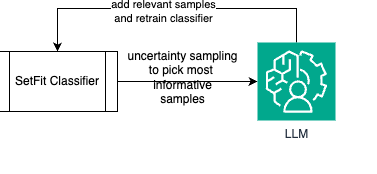
Recursive Expert Delegation: R.E.D.

By doing this, we were able to achieve close-to-human-expert validation numbers on controlled multi-class datasets. Experimentally, R.E.D. scales up to 1,000 classes while maintaining a competent degree of accuracy almost on par with human experts (90%+ agreement).

I believe this is a significant achievement in applied ML, and has real-world uses for production-grade expectations of cost, speed, scale, and adaptability. The technical report, publishing later this year, highlights relevant code samples as well as experimental setups used to achieve given results.

All images, unless otherwise noted, are by the author

Interested in more details? Reach out to me over Medium or email for a chat!

Shape
Shape
Stay Ahead

Explore More Insights

Stay ahead with more perspectives on cutting-edge power, infrastructure, energy,  bitcoin and AI solutions. Explore these articles to uncover strategies and insights shaping the future of industries.

Shape

Akamai acquires Fermyon for edge computing as WebAssembly comes of age

Spin handles compilation from source to WebAssembly bytecode and manages execution on target platforms. The runtime abstracts the underlying technology while preserving WebAssembly’s performance and security characteristics. This bet on WebAssembly standards has paid off as the technology matured.  WebAssembly has evolved significantly beyond its initial browser-focused design to support

Read More »

Winners and losers in the latest Top500 supercomputer list

Winner: Slingshot-11 Slingshot-11 is a 200G proprietary interconnect developed by HPE and its Cray supercomputer subsidiary. As the number of Cray systems increases on the list, so goes the number of Slingshot-11 based systems. The total number of Slingshot-11 systems jumped from 37 and 2024 to 52 this year. Loser:

Read More »

Chevron Joins TotalEnergies in New Nigerian Exploration Blocks

Chevron Corp has signed a deal to acquire 40 percent in Petroleum Prospecting License (PPL) 2000 and PPL 2001 offshore Nigeria from TotalEnergies SE. TotalEnergies will retain operatorship with a 40 percent interest. Local player South Atlantic Petroleum Ltd owns 20 percent. “This new joint venture aims at derisking and

Read More »

Four things AWS needs to fix at re:Invent this week

When it comes to new AI analytics services from AWS, CIOs can expect more of the same, said David Linthicum, independent consultant and retired chief cloud strategy officer at Deloitte Consulting. “Realistically, they can expect AWS to keep integrating its existing services; the key test will be whether this shows

Read More »

Petrogas spuds exploration well onshore Indonesia

Petrogas (Basin) Ltd. spudded the Karim-1 exploration well in the Kepala Burung Production Sharing Contract (PSC), Southwest Papua, Indonesia. The well is being drilled onshore in a relatively under-explored area within Arar block and is about 23 km east of the Petrogas’ existing Arar production cluster. The well will be vertical and drilled to about 1,311 m TD. Drilling and completion is estimated to take 43 days. Karim-1 well is designed to assess the oil potential of the Miocene Kais reservoir within a structural closure located updip of the previous Klaifi-1 oil discovery, situated about 7 km northwest of Karim-1. The Miocene Kais formation is a carbonate sequence that forms a broad shallow marine platform with localized reefal complexes and is the main producing reservoir in the PSC. Following completion of Karim-1 well, the drilling rig will be deployed to drill the Northwest Klagagi-1 exploration well, which is about 15 km northeast of the Arar production cluster and about 12 km from the Karim-1 well site. The Karim-1 well and the Northwest Klagagi-1 well are part of exploration wells being drilled under the firm work commitment of the Kepala Burung PSC which began in 2020. Kepala Burung PSC covers an onshore area of 1,030 sq km within Salawati basin, which is one of the most prolific petroleum basins in Indonesia. Petrogas (Basin) Ltd. is a subsidiary of RH Petrogas Ltd. (82.65% owned). RH Petrogas is operator of the Kepala Burung PSC (70%) with Pertamina holding the remaining 30%.     

Read More »

NextDecade progresses Rio Grande LNG Train 6 plan with FERC pre-filing

@import url(‘https://fonts.googleapis.com/css2?family=Inter:[email protected]&display=swap’); a { color: var(–color-primary-main); } .ebm-page__main h1, .ebm-page__main h2, .ebm-page__main h3, .ebm-page__main h4, .ebm-page__main h5, .ebm-page__main h6 { font-family: Inter; } body { line-height: 150%; letter-spacing: 0.025em; font-family: Inter; } button, .ebm-button-wrapper { font-family: Inter; } .label-style { text-transform: uppercase; color: var(–color-grey); font-weight: 600; font-size: 0.75rem; } .caption-style { font-size: 0.75rem; opacity: .6; } #onetrust-pc-sdk [id*=btn-handler], #onetrust-pc-sdk [class*=btn-handler] { background-color: #c19a06 !important; border-color: #c19a06 !important; } #onetrust-policy a, #onetrust-pc-sdk a, #ot-pc-content a { color: #c19a06 !important; } #onetrust-consent-sdk #onetrust-pc-sdk .ot-active-menu { border-color: #c19a06 !important; } #onetrust-consent-sdk #onetrust-accept-btn-handler, #onetrust-banner-sdk #onetrust-reject-all-handler, #onetrust-consent-sdk #onetrust-pc-btn-handler.cookie-setting-link { background-color: #c19a06 !important; border-color: #c19a06 !important; } #onetrust-consent-sdk .onetrust-pc-btn-handler { color: #c19a06 !important; border-color: #c19a06 !important; } NextDecade Corp. has initiated the pre-filing process with the Federal Energy Regulatory Commission (FERC) for expansion at Rio Grande LNG that includes a sixth liquefaction train (Train 6) and an additional marine berth. The company expects to file a full application for the expansion with FERC in 2026. Trains 1-5 are under construction on the north shore of the Brownsville Ship Channel in south Texas, and NextDecade is developing and advancing the permitting process for Trains 6-8. Train 6 is being developed inside the existing levee at the Rio Grande LNG plant site and adjacent to Trains 1-5. The company is evaluating areas on the site for development of Trains 7 and 8, which would bring potential liquefaction capacity at the plant to about 48 million tonnes/year. NextDecade says the site has sufficient space for development of up to 10 liquefaction trains.

Read More »

Then & Now: Global oil supply transformation

@import url(‘https://fonts.googleapis.com/css2?family=Inter:[email protected]&display=swap’); a { color: var(–color-primary-main); } .ebm-page__main h1, .ebm-page__main h2, .ebm-page__main h3, .ebm-page__main h4, .ebm-page__main h5, .ebm-page__main h6 { font-family: Inter; } body { line-height: 150%; letter-spacing: 0.025em; font-family: Inter; } button, .ebm-button-wrapper { font-family: Inter; } .label-style { text-transform: uppercase; color: var(–color-grey); font-weight: 600; font-size: 0.75rem; } .caption-style { font-size: 0.75rem; opacity: .6; } #onetrust-pc-sdk [id*=btn-handler], #onetrust-pc-sdk [class*=btn-handler] { background-color: #c19a06 !important; border-color: #c19a06 !important; } #onetrust-policy a, #onetrust-pc-sdk a, #ot-pc-content a { color: #c19a06 !important; } #onetrust-consent-sdk #onetrust-pc-sdk .ot-active-menu { border-color: #c19a06 !important; } #onetrust-consent-sdk #onetrust-accept-btn-handler, #onetrust-banner-sdk #onetrust-reject-all-handler, #onetrust-consent-sdk #onetrust-pc-btn-handler.cookie-setting-link { background-color: #c19a06 !important; border-color: #c19a06 !important; } #onetrust-consent-sdk .onetrust-pc-btn-handler { color: #c19a06 !important; border-color: #c19a06 !important; } In this Then & Now episode of the Oil & Gas Journal ReEnterprised podcast, Statistics Editor Laura Bell-Hammer takes listeners on a journey through three decades of oil-market transformation. Bell-Hammer looks back at the mid-1990s, when US production was believed to be in irreversible decline, fast-forwarding to today’s record production highs powered by shale technology, deepwater advances, and new global producers. From the Permian basin to Brazil’s presalt and Guyana’s meteoric rise, this episode reveals how technology reshaped the world’s supply map. OGJ Worldwide Report In this episode of the Oil & Gas Journal ReEnterprised podcast, Bell-Hammer notes OGJ’s annual Worldwide Report, a compilation of field-by-field oil production and country-by-country oil and gas reserves accessible to paid subscribers. The most recent report will be published in December. In the meantime, archived Worldwide Reports can be found as part of OGJ’s Surveys page.  

Read More »

bp Trinidad and Tobago completes Cypre drilling

@import url(‘https://fonts.googleapis.com/css2?family=Inter:[email protected]&display=swap’); a { color: var(–color-primary-main); } .ebm-page__main h1, .ebm-page__main h2, .ebm-page__main h3, .ebm-page__main h4, .ebm-page__main h5, .ebm-page__main h6 { font-family: Inter; } body { line-height: 150%; letter-spacing: 0.025em; font-family: Inter; } button, .ebm-button-wrapper { font-family: Inter; } .label-style { text-transform: uppercase; color: var(–color-grey); font-weight: 600; font-size: 0.75rem; } .caption-style { font-size: 0.75rem; opacity: .6; } #onetrust-pc-sdk [id*=btn-handler], #onetrust-pc-sdk [class*=btn-handler] { background-color: #c19a06 !important; border-color: #c19a06 !important; } #onetrust-policy a, #onetrust-pc-sdk a, #ot-pc-content a { color: #c19a06 !important; } #onetrust-consent-sdk #onetrust-pc-sdk .ot-active-menu { border-color: #c19a06 !important; } #onetrust-consent-sdk #onetrust-accept-btn-handler, #onetrust-banner-sdk #onetrust-reject-all-handler, #onetrust-consent-sdk #onetrust-pc-btn-handler.cookie-setting-link { background-color: #c19a06 !important; border-color: #c19a06 !important; } #onetrust-consent-sdk .onetrust-pc-btn-handler { color: #c19a06 !important; border-color: #c19a06 !important; } bp Trinidad and Tobago (bpTT) completed the Cypre seven-well drilling program 78 km off the southeast coast of Trinidad within East Mayaro block, Columbus basin, in about 80 m of water. The wells are tied back into bpTT’s existing Juniper platform. Four wells were drilled and completed at end-2024 with the first gas delivered in April this year. The project team has now drilled, completed, and commissioned the remaining three wells. At peak, Cypre is projected to deliver about 45,000 boe/d. Cypre is bpTT’s third subsea development and is one of bp’s 10 major projects expected to start up worldwide between 2025 and 2027.  Cypre is 100% owned by bpTT which is owned by bp (70%) and Repsol (30%).

Read More »

Shell adds 10% stake in operated field offshore Nigeria as Eni exercises preemption right

@import url(‘https://fonts.googleapis.com/css2?family=Inter:[email protected]&display=swap’); a { color: var(–color-primary-main); } .ebm-page__main h1, .ebm-page__main h2, .ebm-page__main h3, .ebm-page__main h4, .ebm-page__main h5, .ebm-page__main h6 { font-family: Inter; } body { line-height: 150%; letter-spacing: 0.025em; font-family: Inter; } button, .ebm-button-wrapper { font-family: Inter; } .label-style { text-transform: uppercase; color: var(–color-grey); font-weight: 600; font-size: 0.75rem; } .caption-style { font-size: 0.75rem; opacity: .6; } #onetrust-pc-sdk [id*=btn-handler], #onetrust-pc-sdk [class*=btn-handler] { background-color: #c19a06 !important; border-color: #c19a06 !important; } #onetrust-policy a, #onetrust-pc-sdk a, #ot-pc-content a { color: #c19a06 !important; } #onetrust-consent-sdk #onetrust-pc-sdk .ot-active-menu { border-color: #c19a06 !important; } #onetrust-consent-sdk #onetrust-accept-btn-handler, #onetrust-banner-sdk #onetrust-reject-all-handler, #onetrust-consent-sdk #onetrust-pc-btn-handler.cookie-setting-link { background-color: #c19a06 !important; border-color: #c19a06 !important; } #onetrust-consent-sdk .onetrust-pc-btn-handler { color: #c19a06 !important; border-color: #c19a06 !important; } Shell Nigeria Exploration and Production Co. (SNEPCo), a subsidiary of Shell plc, has added 10% interest to its stake in Bonga field offshore Nigeria. The now-completed deal with TotalEnergies EP Nigeria Ltd. brings Shell’s stake in the OML 118 production sharing contract to 65% from 55%, a slight decrease in the total expected stake as Eni SpA subsidiary Nigeria Agip Exploration Ltd. (NAE) exercised its preemption right to acquire a 2.5% stake from TotalEnergies’ 12.5% share. SNEPCo (65%) operates Bonga field in partnership with Esso Exploration and Production Nigeria Ltd. (20%), and NAE (15%), on behalf of the Nigerian National Petroleum Co. Ltd. (NNPC). Bonga field lies in the Gulf of Guinea about 120 km south of the Niger Delta in water depths over 1,000 m. The field is produced via a floating production storage and offloading (FPSO) vessel with capacity to produce 225,000 b/d of oil. Last year, SNEPCo took final investment decision (FID) to develop Bonga North via subsea tieback to the FPSO.   

Read More »

FERC grants extension to Sempra’s Cameron LNG, explores certain blanket LNG plant authorizations

The US Federal Energy Regulatory Commission (FERC) Nov. 23 granted Sempra Infrastructure a 5-year extension to construct and place into service its planned 6.75 million tonne/year Cameron LNG plant in Cameron Parish, La. FERC’s new certificate extends the plant’s start date to Mar. 16, 2033. Sempra in October requested FERC push the deadline, noting that “project lenders require assurances that it has all necessary authorizations, including the approval of this extension of time request prior to reaching a positive financial decision” for the plant, according to FERC’s order. FERC noted that Sempra had reported progress working with the Louisiana Department of Environmental Quality (LDEQ). Sempra described “significant engineering and commercial efforts to advance the project such as various design enhancements to increase efficiency and reliability of the project” in its filing, FERC said. FERC notice of inquiry Meanwhile, FERC Nov. 20 took the first steps to streamline approvals of LNG plants by requesting comments on whether the commission should establish blanket authorization for certain activities at the plants. Law firm Van Ness Feldman, in a client alert Nov. 24, called FERC’s notice of inquiry (NOI) “significant,” especially given the  rapid growth of the US LNG sector. A blanket authorization program for LNG plants “could expedite certain modifications and expansions, reduce regulatory burdens and provide greater certainty for project developers,” the alert said. FERC has maintained a blanket certificate program for interstate natural gas pipelines since 1982. Under the program, interstate pipeline owners can perform certain routine activities without individual authorization, provided they meet regulatory requirements and cost limits. In the past, FERC declined to extend blanket authorization to LNG plants, citing environmental and security concerns and highlighting the non-routine nature of LNG projects at the time. In the NOI, FERC said its “experience with LNG facilities in the United States

Read More »

Nvidia’s $2B Synopsys stake tests independence of open AI interconnect standard

But the concern for enterprise IT leaders is whether Nvidia’s financial stakes in UALink consortium members could influence the development of an open standard specifically designed to compete with Nvidia’s proprietary technology and to give enterprises more choices in the datacenter. Organizations planning major AI infrastructure investments view such open standards as critical to avoiding vendor lock-in and maintaining competitive pricing. “This does put more pressure on UALink since Intel is also a member and also took investment from Nvidia,” Sag said. UALink and Synopsys’s critical role UALink represents the industry’s most significant effort to prevent vendor lock-in for AI infrastructure. The consortium ratified its UALink 200G 1.0 Specification in April, defining an open standard for connecting up to 1,024 AI accelerators within computing pods at 200 Gbps per lane — directly competing with Nvidia’s NVLink for scale-up applications. Synopsys plays a critical role. The company joined UALink’s board in January and in December announced the industry’s first UALink design components, enabling chip designers to build UALink-compatible accelerators. Analysts flag governance concerns Gaurav Gupta, VP analyst at Gartner, acknowledged the tension. “The Nvidia-Synopsys deal does raise questions around the future of UALink as Synopsys is a key partner of the consortium and holds critical IP for UALink, which competes with Nvidia’s proprietary NVLink,” he said. Sanchit Vir Gogia, chief analyst at Greyhound Research, sees deeper structural concerns. “Synopsys is not a peripheral player in this standard; it is the primary supplier of UALink IP and a board member within the UALink Consortium,” he said. “Nvidia’s entry into Synopsys’ shareholder structure risks contaminating that neutrality.”

Read More »

Cooling crisis at CME: A wakeup call for modern infrastructure governance

Organizations should reassess redundancy However, he pointed out, “the deeper concern is that CME had a secondary data center ready to take the load, yet the failover threshold was set too high, and the activation sequence remained manually gated. The decision to wait for the cooling issue to self-correct rather than trigger the backup site immediately revealed a governance model that had not evolved to keep pace with the operational tempo of modern markets.” Thermal failures, he said, “do not unfold on the timelines assumed in traditional disaster recovery playbooks. They escalate within minutes and demand automated responses that do not depend on human certainty about whether a facility will recover in time.” Matt Kimball, VP and principal analyst at Moor Insights & Strategy, said that to some degree what happened in Aurora highlights an issue that may arise on occasion: “the communications gap that can exist between IT executives and data center operators. Think of ‘rack in versus rack out’ mindsets.” Often, he said, the operational elements of that data center environment, such as cooling, power, fire hazards, physical security, and so forth, fall outside the realm of an IT executive focused on delivering IT services to the business. “And even if they don’t fall outside the realm, these elements are certainly not a primary focus,” he noted. “This was certainly true when I was living in the IT world.” Additionally, said Kimball, “this highlights the need for organizations to reassess redundancy and resilience in a new light. Again, in IT, we tend to focus on resilience and redundancy at the app, server, and workload layers. Maybe even cluster level. But as we continue to place more and more of a premium on data, and the terms ‘business critical’ or ‘mission critical’ have real relevance, we have to zoom out

Read More »

Microsoft loses two senior AI infrastructure leaders as data center pressures mount

Microsoft did not immediately respond to a request for comment. Microsoft’s constraints Analysts say the twin departures mark a significant setback for Microsoft at a critical moment in the AI data center race, with pressure mounting from both OpenAI’s model demands and Google’s infrastructure scale. “Losing some of the best professionals working on this challenge could set Microsoft back,” said Neil Shah, partner and co-founder at Counterpoint Research. “Solving the energy wall is not trivial, and there may have been friction or strategic differences that contributed to their decision to move on, especially if they saw an opportunity to make a broader impact and do so more lucratively at a company like Nvidia.” Even so, Microsoft has the depth and ecosystem strength to continue doubling down on AI data centers, said Prabhu Ram, VP for industry research at Cybermedia Research. According to Sanchit Gogia, chief analyst at Greyhound Research, the departures come at a sensitive moment because Microsoft is trying to expand its AI infrastructure faster than physical constraints allow. “The executives who have left were central to GPU cluster design, data center engineering, energy procurement, and the experimental power and cooling approaches Microsoft has been pursuing to support dense AI workloads,” Gogia said. “Their exit coincides with pressures the company has already acknowledged publicly. GPUs are arriving faster than the company can energize the facilities that will house them, and power availability has overtaken chip availability as the real bottleneck.”

Read More »

What is Edge AI? When the cloud isn’t close enough

Many edge devices can periodically send summarized or selected inference output data back to a central system for model retraining or refinement. That feedback loop helps the model improve over time while still keeping most decisions local. And to run efficiently on constrained edge hardware, the AI model is often pre-processed by techniques such as quantization (which reduces precision), pruning (which removes redundant parameters), or knowledge distillation (which trains a smaller model to mimic a larger one). These optimizations reduce the model’s memory, compute, and power demands so it can run more easily on an edge device. What technologies make edge AI possible? The concept of the “edge” always assumes that edge devices are less computationally powerful than data centers and cloud platforms. While that remains true, overall improvements in computational hardware have made today’s edge devices much more capable than those designed just a few years ago. In fact, a whole host of technological developments have come together to make edge AI a reality. Specialized hardware acceleration. Edge devices now ship with dedicated AI-accelerators (NPUs, TPUs, GPU cores) and system-on-chip units tailored for on-device inference. For example, companies like Arm have integrated AI-acceleration libraries into standard frameworks so models can run efficiently on Arm-based CPUs. Connectivity and data architecture. Edge AI often depends on durable, low-latency links (e.g., 5G, WiFi 6, LPWAN) and architectures that move compute closer to data. Merging edge nodes, gateways, and local servers means less reliance on distant clouds. And technologies like Kubernetes can provide a consistent management plane from the data center to remote locations. Deployment, orchestration, and model lifecycle tooling. Edge AI deployments must support model-update delivery, device and fleet monitoring, versioning, rollback and secure inference — especially when orchestrated across hundreds or thousands of locations. VMware, for instance, is offering traffic management

Read More »

Networks, AI, and metaversing

Our first, conservative, view says that AI’s network impact is largely confined to the data center, to connect clusters of GPU servers and the data they use as they crunch large language models. It’s all “horizontal” traffic; one TikTok challenge would generate way more traffic in the wide area. WAN costs won’t rise for you as an enterprise, and if you’re a carrier you won’t be carrying much new, so you don’t have much service revenue upside. If you don’t host AI on premises, you can pretty much dismiss its impact on your network. Contrast that with the radical metaverse view, our third view. Metaverses and AR/VR transform AI missions, and network services, from transaction processing to event processing, because the real world is a bunch of events pushing on you. They also let you visualize the way that process control models (digital twins) relate to the real world, which is critical if the processes you’re modeling involve human workers who rely on their visual sense. Could it be that the reason Meta is willing to spend on AI, is that the most credible application of AI, and the most impactful for networks, is the metaverse concept? In any event, this model of AI, by driving the users’ experiences and activities directly, demands significant edge connectivity, so you could expect it to have a major impact on network requirements. In fact, just dipping your toes into a metaverse could require a major up-front network upgrade. Networks carry traffic. Traffic is messages. More messages, more traffic, more infrastructure, more service revenue…you get the picture. Door number one, to the AI giant future, leads to nothing much in terms of messages. Door number three, metaverses and AR/VR, leads to a message, traffic, and network revolution. I’ll bet that most enterprises would doubt

Read More »

Microsoft’s Fairwater Atlanta and the Rise of the Distributed AI Supercomputer

Microsoft’s second Fairwater data center in Atlanta isn’t just “another big GPU shed.” It represents the other half of a deliberate architectural experiment: proving that two massive AI campuses, separated by roughly 700 miles, can operate as one coherent, distributed supercomputer. The Atlanta installation is the latest expression of Microsoft’s AI-first data center design: purpose-built for training and serving frontier models rather than supporting mixed cloud workloads. It links directly to the original Fairwater campus in Wisconsin, as well as to earlier generations of Azure AI supercomputers, through a dedicated AI WAN backbone that Microsoft describes as the foundation of a “planet-scale AI superfactory.” Inside a Fairwater Site: Preparing for Multi-Site Distribution Efficient multi-site training only works if each individual site behaves as a clean, well-structured unit. Microsoft’s intra-site design is deliberately simplified so that cross-site coordination has a predictable abstraction boundary—essential for treating multiple campuses as one distributed AI system. Each Fairwater installation presents itself as a single, flat, high-regularity cluster: Up to 72 NVIDIA Blackwell GPUs per rack, using GB200 NVL72 rack-scale systems. NVLink provides the ultra-low-latency, high-bandwidth scale-up fabric within the rack, while the Spectrum-X Ethernet stack handles scale-out. Each rack delivers roughly 1.8 TB/s of GPU-to-GPU bandwidth and exposes a multi-terabyte pooled memory space addressable via NVLink—critical for large-model sharding, activation checkpointing, and parallelism strategies. Racks feed into a two-tier Ethernet scale-out network offering 800 Gbps GPU-to-GPU connectivity with very low hop counts, engineered to scale to hundreds of thousands of GPUs without encountering the classic port-count and topology constraints of traditional Clos fabrics. Microsoft confirms that the fabric relies heavily on: SONiC-based switching and a broad commodity Ethernet ecosystem to avoid vendor lock-in and accelerate architectural iteration. Custom network optimizations, such as packet trimming, packet spray, high-frequency telemetry, and advanced congestion-control mechanisms, to prevent collective

Read More »

Microsoft will invest $80B in AI data centers in fiscal 2025

And Microsoft isn’t the only one that is ramping up its investments into AI-enabled data centers. Rival cloud service providers are all investing in either upgrading or opening new data centers to capture a larger chunk of business from developers and users of large language models (LLMs).  In a report published in October 2024, Bloomberg Intelligence estimated that demand for generative AI would push Microsoft, AWS, Google, Oracle, Meta, and Apple would between them devote $200 billion to capex in 2025, up from $110 billion in 2023. Microsoft is one of the biggest spenders, followed closely by Google and AWS, Bloomberg Intelligence said. Its estimate of Microsoft’s capital spending on AI, at $62.4 billion for calendar 2025, is lower than Smith’s claim that the company will invest $80 billion in the fiscal year to June 30, 2025. Both figures, though, are way higher than Microsoft’s 2020 capital expenditure of “just” $17.6 billion. The majority of the increased spending is tied to cloud services and the expansion of AI infrastructure needed to provide compute capacity for OpenAI workloads. Separately, last October Amazon CEO Andy Jassy said his company planned total capex spend of $75 billion in 2024 and even more in 2025, with much of it going to AWS, its cloud computing division.

Read More »

John Deere unveils more autonomous farm machines to address skill labor shortage

Join our daily and weekly newsletters for the latest updates and exclusive content on industry-leading AI coverage. Learn More Self-driving tractors might be the path to self-driving cars. John Deere has revealed a new line of autonomous machines and tech across agriculture, construction and commercial landscaping. The Moline, Illinois-based John Deere has been in business for 187 years, yet it’s been a regular as a non-tech company showing off technology at the big tech trade show in Las Vegas and is back at CES 2025 with more autonomous tractors and other vehicles. This is not something we usually cover, but John Deere has a lot of data that is interesting in the big picture of tech. The message from the company is that there aren’t enough skilled farm laborers to do the work that its customers need. It’s been a challenge for most of the last two decades, said Jahmy Hindman, CTO at John Deere, in a briefing. Much of the tech will come this fall and after that. He noted that the average farmer in the U.S. is over 58 and works 12 to 18 hours a day to grow food for us. And he said the American Farm Bureau Federation estimates there are roughly 2.4 million farm jobs that need to be filled annually; and the agricultural work force continues to shrink. (This is my hint to the anti-immigration crowd). John Deere’s autonomous 9RX Tractor. Farmers can oversee it using an app. While each of these industries experiences their own set of challenges, a commonality across all is skilled labor availability. In construction, about 80% percent of contractors struggle to find skilled labor. And in commercial landscaping, 86% of landscaping business owners can’t find labor to fill open positions, he said. “They have to figure out how to do

Read More »

2025 playbook for enterprise AI success, from agents to evals

Join our daily and weekly newsletters for the latest updates and exclusive content on industry-leading AI coverage. Learn More 2025 is poised to be a pivotal year for enterprise AI. The past year has seen rapid innovation, and this year will see the same. This has made it more critical than ever to revisit your AI strategy to stay competitive and create value for your customers. From scaling AI agents to optimizing costs, here are the five critical areas enterprises should prioritize for their AI strategy this year. 1. Agents: the next generation of automation AI agents are no longer theoretical. In 2025, they’re indispensable tools for enterprises looking to streamline operations and enhance customer interactions. Unlike traditional software, agents powered by large language models (LLMs) can make nuanced decisions, navigate complex multi-step tasks, and integrate seamlessly with tools and APIs. At the start of 2024, agents were not ready for prime time, making frustrating mistakes like hallucinating URLs. They started getting better as frontier large language models themselves improved. “Let me put it this way,” said Sam Witteveen, cofounder of Red Dragon, a company that develops agents for companies, and that recently reviewed the 48 agents it built last year. “Interestingly, the ones that we built at the start of the year, a lot of those worked way better at the end of the year just because the models got better.” Witteveen shared this in the video podcast we filmed to discuss these five big trends in detail. Models are getting better and hallucinating less, and they’re also being trained to do agentic tasks. Another feature that the model providers are researching is a way to use the LLM as a judge, and as models get cheaper (something we’ll cover below), companies can use three or more models to

Read More »

OpenAI’s red teaming innovations define new essentials for security leaders in the AI era

Join our daily and weekly newsletters for the latest updates and exclusive content on industry-leading AI coverage. Learn More OpenAI has taken a more aggressive approach to red teaming than its AI competitors, demonstrating its security teams’ advanced capabilities in two areas: multi-step reinforcement and external red teaming. OpenAI recently released two papers that set a new competitive standard for improving the quality, reliability and safety of AI models in these two techniques and more. The first paper, “OpenAI’s Approach to External Red Teaming for AI Models and Systems,” reports that specialized teams outside the company have proven effective in uncovering vulnerabilities that might otherwise have made it into a released model because in-house testing techniques may have missed them. In the second paper, “Diverse and Effective Red Teaming with Auto-Generated Rewards and Multi-Step Reinforcement Learning,” OpenAI introduces an automated framework that relies on iterative reinforcement learning to generate a broad spectrum of novel, wide-ranging attacks. Going all-in on red teaming pays practical, competitive dividends It’s encouraging to see competitive intensity in red teaming growing among AI companies. When Anthropic released its AI red team guidelines in June of last year, it joined AI providers including Google, Microsoft, Nvidia, OpenAI, and even the U.S.’s National Institute of Standards and Technology (NIST), which all had released red teaming frameworks. Investing heavily in red teaming yields tangible benefits for security leaders in any organization. OpenAI’s paper on external red teaming provides a detailed analysis of how the company strives to create specialized external teams that include cybersecurity and subject matter experts. The goal is to see if knowledgeable external teams can defeat models’ security perimeters and find gaps in their security, biases and controls that prompt-based testing couldn’t find. What makes OpenAI’s recent papers noteworthy is how well they define using human-in-the-middle

Read More »