This is the first article in a series dedicated to Deep Learning, a group of Machine Learning methods that has its roots dating back to the 1940’s. Deep Learning gained attention in the last decades for its groundbreaking application in areas like image classification, speech recognition, and machine translation.
Stay tuned if you’d like to see different Deep Learning algorithms explained with real-life examples and some Python code.
This series of articles focuses on Deep Learning algorithms, which have been getting a lot of attention in the last few years, as many of its applications take center stage in our day-to-day life. From self-driving cars to voice assistants, face recognition or the ability to transcribe speech into text.
These applications are just the tip of the iceberg. A long path of research and incremental applications has been paved since the early 1940’s. The improvements and widespread applications we’re seeing today are the culmination of the hardware and data availability catching up with computational demands of these complex methods.
In traditional Machine Learning anyone who is building a model either has to be an expert in the problem area they are working on, or team up with one. Without this expert knowledge, designing and engineering features becomes an increasingly difficult challenge[1]. The quality of a Machine Learning model depends on the quality of the dataset, but also on how well features encode the patterns in the data.
Deep Learning algorithms use Artificial Neural Networks as their main structure. What sets them apart from other algorithms is that they don’t require expert input during the feature design and engineering phase. Neural Networks can learn the characteristics of the data.
Deep Learning algorithms take in the dataset and learn its patterns, they learn how to represent the data with features they extract on their own. Then they combine different representations of the dataset, each one identifying a specific pattern or characteristic, into a more abstract, high-level representation of the dataset[1]. This hands-off approach, without much human intervention in feature design and extraction, allows algorithms to adapt much faster to the data at hand[2].
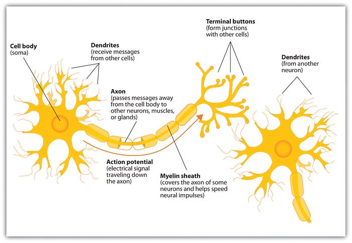
Neural Networks are inspired by, but not necessarily an exact model of, the structure of the brain. There’s a lot we still don’t know about the brain and how it works, but it has been serving as inspiration in many scientific areas due to its ability to develop intelligence. And although there are neural networks that were created with the sole purpose of understanding how brains work, Deep Learning as we know it today is not intended to replicate how the brain works. Instead, Deep Learning focuses on enabling systems that learn multiple levels of pattern composition[1].
And, as with any scientific progress, Deep Learning didn’t start off with the complex structures and widespread applications you see in recent literature.
It all started with a basic structure, one that resembles brain’s neuron.
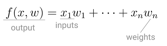
In the early 1940’s Warren McCulloch, a neurophysiologist, teamed up with logician Walter Pitts to create a model of how brains work. It was a simple linear model that produced a positive or negative output, given a set of inputs and weights.
This model of computation was intentionally called neuron, because it tried to mimic how the core building block of the brain worked. Just like brain neurons receive electrical signals, McCulloch and Pitts’ neuron received inputs and, if these signals were strong enough, passed them on to other neurons.
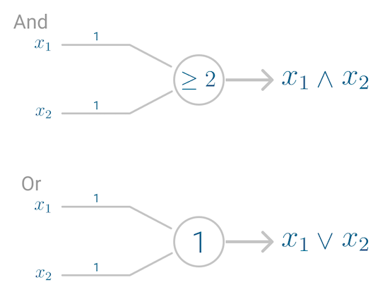
The first application of the neuron replicated a logic gate, where you have one or two binary inputs, and a boolean function that only gets activated given the right inputs and weights.
However, this model had a problem. It couldn’t learn like the brain. The only way to get the desired output was if the weights, working as catalyst in the model, were set beforehand.
The nervous system is a net of neurons, each having a soma and an axon […] At any instant a neuron has some threshold, which excitation must exceed to initiate an impulse[3].
It was only a decade later that Frank Rosenblatt extended this model, and created an algorithm that could learn the weights in order to generate an output.
Building onto McCulloch and Pitt’s neuron, Rosenblatt developed the Perceptron.
Although today the Perceptron is widely recognized as an algorithm, it was initially intended as an image recognition machine. It gets its name from performing the human-like function of perception, seeing and recognizing images.
In particular, interest has been centered on the idea of a machine which would be capable of conceptualizing inputs impinging directly from the physical environment of light, sound, temperature, etc. — the “phenomenal world” with which we are all familiar — rather than requiring the intervention of a human agent to digest and code the necessary information.[4]
Rosenblatt’s perceptron machine relied on a basic unit of computation, the neuron. Just like in previous models, each neuron has a cell that receives a series of pairs of inputs and weights.
The major difference in Rosenblatt’s model is that inputs are combined in a weighted sum and, if the weighted sum exceeds a predefined threshold, the neuron fires and produces an output.
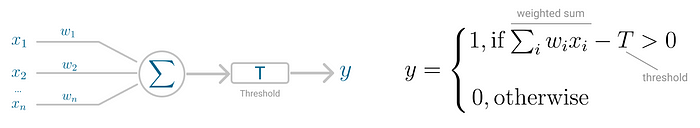
Threshold T represents the activation function. If the weighted sum of the inputs is greater than zero the neuron outputs the value 1, otherwise the output value is zero.
With this discrete output, controlled by the activation function, the perceptron can be used as a binary classification model, defining a linear decision boundary. It finds the separating hyperplane that minimizes the distance between misclassified points and the decision boundary[6].
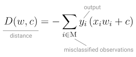
To minimize this distance, Perceptron uses Stochastic Gradient Descent as the optimization function.
If the data is linearly separable, it is guaranteed that Stochastic Gradient Descent will converge in a finite number of steps.
The last piece that Perceptron needs is the activation function, the function that determines if the neuron will fire or not.
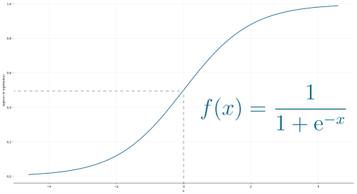
Initial Perceptron models used sigmoid function, and just by looking at its shape, it makes a lot of sense!
The sigmoid function maps any real input to a value that is either 0 or 1, and encodes a non-linear function.
The neuron can receive negative numbers as input, and it will still be able to produce an output that is either 0 or 1.
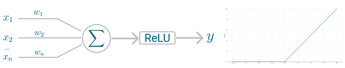
But, if you look at Deep Learning papers and algorithms from the last decade, you’ll see the most of them use the Rectified Linear Unit (ReLU) as the neuron’s activation function.
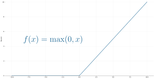
The reason why ReLU became more adopted is that it allows better optimization using Stochastic Gradient Descent, more efficient computation and is scale-invariant, meaning, its characteristics are not affected by the scale of the input.
Putting it all together
The neuron receives inputs and picks an initial set of weights a random. These are combined in weighted sum and then ReLU, the activation function, determines the value of the output.
But you might be wondering, Doesn’t Perceptron actually learn the weights?
It does! Perceptron uses Stochastic Gradient Descent to find, or you might say learn, the set of weight that minimizes the distance between the misclassified points and the decision boundary. Once Stochastic Gradient Descent converges, the dataset is separated into two regions by a linear hyperplane.
Although it was said the Perceptron could represent any circuit and logic, the biggest criticism was that it couldn’t represent the XOR gate, exclusive OR, where the gate only returns 1 if the inputs are different.
This was proved almost a decade later by Minsky and Papert, in 1969[5] and highlights the fact that Perceptron, with only one neuron, can’t be applied to non-linear data.
The Multilayer Perceptron was developed to tackle this limitation. It is a neural network where the mapping between inputs and output is non-linear.
A Multilayer Perceptron has input and output layers, and one or more hidden layers with many neurons stacked together. And while in the Perceptron the neuron must have an activation function that imposes a threshold, like ReLU or sigmoid, neurons in a Multilayer Perceptron can use any arbitrary activation function.
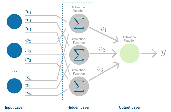
Multilayer Perceptron falls under the category of feedforward algorithms, because inputs are combined with the initial weights in a weighted sum and subjected to the activation function, just like in the Perceptron. But the difference is that each linear combination is propagated to the next layer.
Each layer is feeding the next one with the result of their computation, their internal representation of the data. This goes all the way through the hidden layers to the output layer.
But it has more to it.
If the algorithm only computed the weighted sums in each neuron, propagated results to the output layer, and stopped there, it wouldn’t be able to learn the weights that minimize the cost function. If the algorithm only computed one iteration, there would be no actual learning.
This is where Backpropagation[7] comes into play.
Backpropagation is the learning mechanism that allows the Multilayer Perceptron to iteratively adjust the weights in the network, with the goal of minimizing the cost function.
There is one hard requirement for backpropagation to work properly. The function that combines inputs and weights in a neuron, for instance the weighted sum, and the threshold function, for instance ReLU, must be differentiable. These functions must have a bounded derivative, because Gradient Descent is typically the optimization function used in MultiLayer Perceptron.
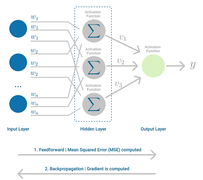
In each iteration, after the weighted sums are forwarded through all layers, the gradient of the Mean Squared Error is computed across all input and output pairs. Then, to propagate it back, the weights of the first hidden layer are updated with the value of the gradient. That’s how the weights are propagated back to the starting point of the neural network!
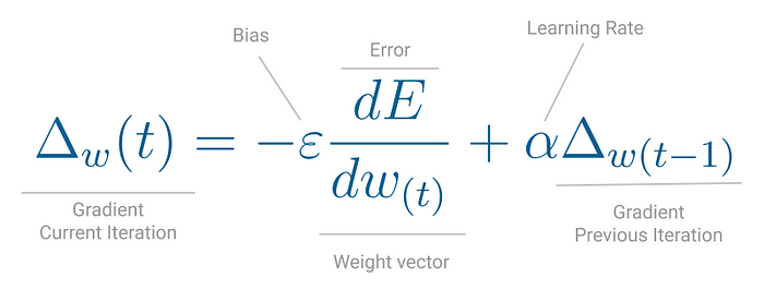
This process keeps going until gradient for each input-output pair has converged, meaning the newly computed gradient hasn’t changed more than a specified convergence threshold, compared to the previous iteration.
Let’s see this with a real-world example.
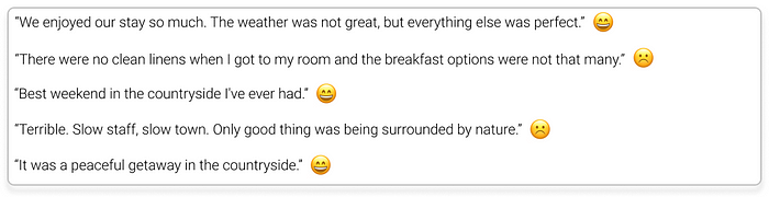
Your parents have a cozy bed and breakfast in the countryside with the traditional guestbook in the lobby. Every guest is welcome to write a note before they leave and, so far, very few leave without writing a short note or inspirational quote. Some even leave drawings of Molly, the family dog.
Summer season is getting to a close, which means cleaning time, before work starts picking up again for the holidays. In the old storage room, you’ve stumbled upon a box full of guestbooks your parents kept over the years. Your first instinct? Let’s read everything!
After reading a few pages, you just had a much better idea. Why not try to understand if guests left a positive or negative message?
You’re a Data Scientist, so this is the perfect task for a binary classifier.
So you picked a handful of guestbooks at random, to use as training set, transcribed all the messages, gave it a classification of positive or negative sentiment, and then asked your cousins to classify them as well.
In Natural Language Processing tasks, some of the text can be ambiguous, so usually you have a corpus of text where the labels were agreed upon by 3 experts, to avoid ties.
With the final labels assigned to the entire corpus, you decided to fit the data to a Perceptron, the simplest neural network of all.
But before building the model itself, you needed to turn that free text into a format the Machine Learning model could work with.
In this case, you represented the text from the guestbooks as a vector using the Term Frequency — Inverse Document Frequency (TF-IDF). This method encodes any kind of text as a statistic of how frequent each word, or term, is in each sentence and the entire document.
In Python you used TfidfVectorizer method from ScikitLearn, removing English stop-words and even applying L1 normalization.
TfidfVectorizer(stop_words='english', lowercase=True, norm='l1')On to binary classification with Perceptron!
To accomplish this, you used Perceptron completely out-of-the-box, with all the default parameters.
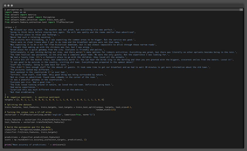
After vectorizing the corpus and fitting the model and testing on sentences the model has never seen before, you realize the Mean Accuracy of this model is 67%.
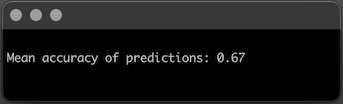
That’s not bad for a simple neural network like Perceptron!
On average, Perceptron will misclassify roughly 1 in every 3 messages your parents’ guests wrote. Which makes you wonder if perhaps this data is not linearly separable and that you could also achieve a better result with a slightly more complex neural network.
Using SckitLearn’s MultiLayer Perceptron, you decided to keep it simple and tweak just a few parameters:
- Activation function: ReLU, specified with the parameter activation=’relu’
- Optimization function: Stochastic Gradient Descent, specified with the parameter solver=’sgd’
- Learning rate: Inverse Scaling, specified with the parameter learning_rate=’invscaling’
- Number of iterations: 20, specified with the parameter max_iter=20
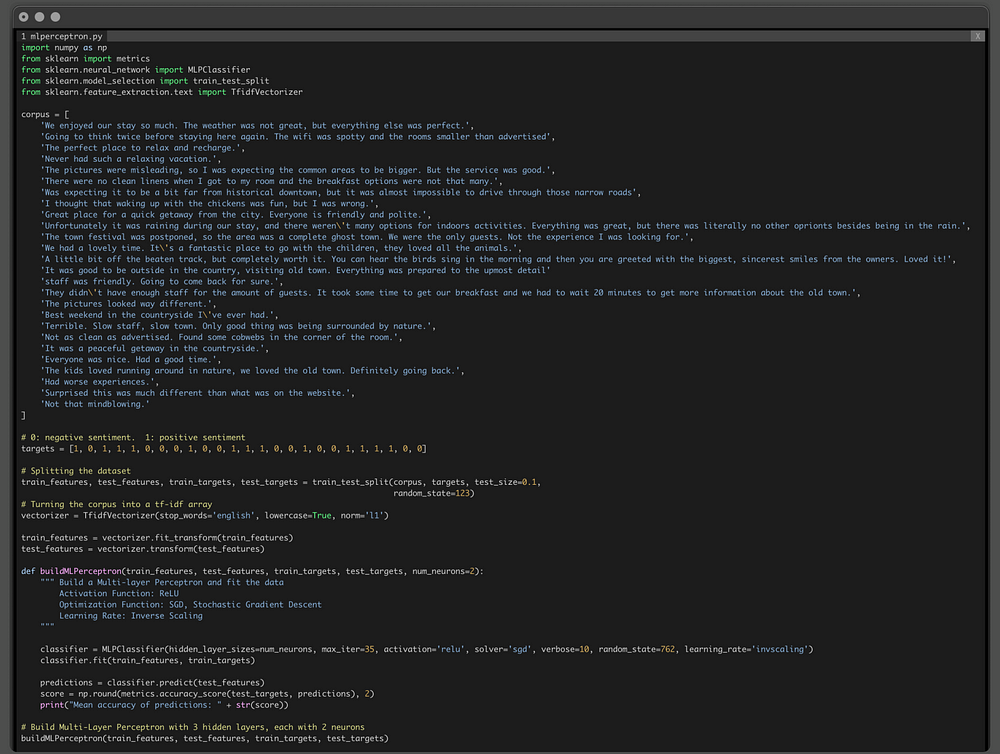
By default, Multilayer Perceptron has three hidden layers, but you want to see how the number of neurons in each layer impacts performance, so you start off with 2 neurons per hidden layer, setting the parameter num_neurons=2.
Finally, to see the value of the loss function at each iteration, you also added the parameter verbose=True.
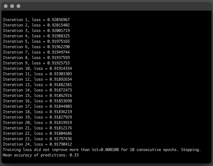
In this case, the Multilayer Perceptron has 3 hidden layers with 2 nodes each, performs much worse than a simple Perceptron.
It converges relatively fast, in 24 iterations, but the mean accuracy is not good.
While the Perceptron misclassified on average 1 in every 3 sentences, this Multilayer Perceptron is kind of the opposite, on average predicts the correct label 1 in every 3 sentences.
What about if you added more capacity to the neural network? What happens when each hidden layer has more neurons to learn the patterns of the dataset?
Using the same method, you can simply change the num_neurons parameter an set it, for instance, to 5.
buildMLPerceptron(train_features, test_features, train_targets, test_targets, num_neurons=5)Adding more neurons to the hidden layers definitely improved Model accuracy!
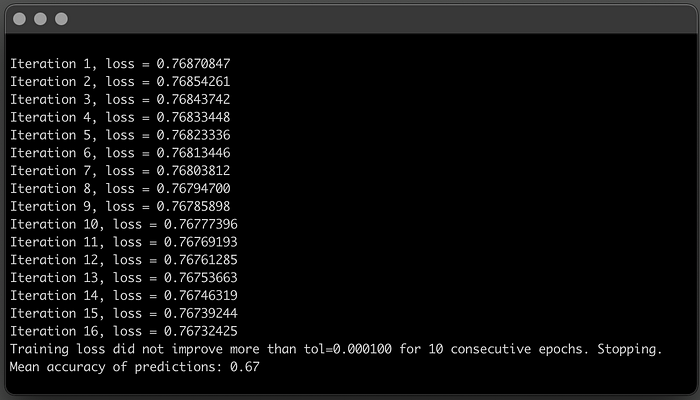
You kept the same neural network structure, 3 hidden layers, but with the increased computational power of the 5 neurons, the model got better at understanding the patterns in the data. It converged much faster and mean accuracy doubled!
In the end, for this specific case and dataset, the Multilayer Perceptron performs as well as a simple Perceptron. But it was definitely a great exercise to see how changing the number of neurons in each hidden-layer impacts model performance.
It’s not a perfect model, there’s possibly some room for improvement, but the next time a guest leaves a message that your parents are not sure if it’s positive or negative, you can use Perceptron to get a second opinion.
The first Deep Learning algorithm was very simple, compared to the current state-of-the-art. Perceptron is a neural network with only one neuron, and can only understand linear relationships between the input and output data provided.
However, with Multilayer Perceptron, horizons are expanded and now this neural network can have many layers of neurons, and ready to learn more complex patterns.
Hope you’ve enjoyed learning about algorithms!
Stay tuned for the next articles in this series, where we continue to explore Deep Learning algorithms.
- LeCun, Y., Bengio, Y. & Hinton, G. Deep learning. Nature 521, 436–444 (2015)
- Ian Goodfellow, Yoshua Bengio, and Aaron Courville. 2016. Deep Learning. The MIT Press.
- McCulloch, W.S., Pitts, W. A logical calculus of the ideas immanent in nervous activity. Bulletin of Mathematical Biophysics 5, 115–133 (1943)
- Frank Rosenblatt. The Perceptron, a Perceiving and Recognizing Automaton Project Para. Cornell Aeronautical Laboratory 85, 460–461 (1957)
- Minsky M. L. and Papert S. A. 1969. Perceptrons. Cambridge, MA: MIT Press.
- Gareth James, Daniela Witten, Trevor Hastie, Robert Tibshirani. (2013). An introduction to statistical learning : with applications in R. New York :Springer
- D. Rumelhart, G. Hinton, and R. Williams. Learning Representations by Back-propagating Errors. Nature 323 (6088): 533–536 (1986).