At some point or another, any Power BI developer must write complex Dax expressions to analyze data. But nobody tells you how to do it. What’s the process for doing it? What is the best way to do it, and how supportive can a development process be? These are the questions I will answer here.
Introduction
Sometimes my clients ask me how I came up with the solution for a specific measure in DAX. My answer is always that I follow a specific process to find a solution.
Sometimes, the process is not straightforward, and I must deviate or start from scratch when I see that I have taken the wrong direction.
But the development process is always the same:
1. Understand the requirements.
2. Define the math to calculate the result.
3. Understand if the measure must work in any or one specific scenario.
4. Start with intermediary results and work my way step-by-step until I fully understand how it should work and can deliver the requested result.
5. Calculate the final result.
The third step is the most difficult.
Sometimes my client asks me to calculate a specific result in a particular scenario. But after I ask again, the answer is: Yes, I will also use it in other scenarios.
For example, some time ago, a client asked me to create some measures for a specific scenario in a report. I had to do it live during a workshop with the client’s team.
Days after I delivered the requested results, he asked me to create another report based on the same semantic model and logic we elaborated on during the workshop, but for a more flexible scenario.
The first set of measures was designed to work tightly with the first scenario, so I didn’t want to change them. Therefore, I created a new set of more generic measures.
Yes, this is a worst-case scenario, but it is something that can happen.
This was just an example of how important it is to take some time to thoroughly understand the needs and the possible future use cases for the requested measures.
Step 1: The requirements
For this piece, I take one measure from my previous article to calculate the linear extrapolation of my customer count.
The requirements are:
- Use the Customer Count Measure as the Basis Measure.
- The user can select the year to analyze.
- The user can select any other dimension in any Slicer.
- The User will analyze the result over time per month.
- The past Customer Count should be taken as the input values.
- The YTD growth rate must be used as the basis for the result.
- Based on the YTD growth rate, the Customer Count should be extrapolated to the end of the year.
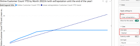
- The YTD Customer Count and the Extrapolation must be shown on the same Line-Chart.
The result should look like this for the year 2022:
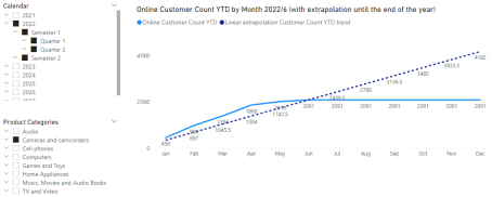
OK, let’s look at how I developed this measure.
But before doing so, we must understand what the filter context is.
If you are already familiar with it, you can skip this section. Or you can read it anyway to ensure we are at the same level.
Interlude: The filter context
The filter context is the central concept of DAX.
When writing measures in a semantic model, whether in Power Bi, a fabric semantic model, or an analysis services semantic model, you must always understand the current filter context.
The filter context is:
The sum of all Filters which affect the result of a DAX expression.
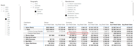
Look at the following picture:
Now, look at the following picture:
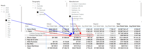
There are six filters, that affect the filter context of the marked cells for the two measures “Sum Retail Sales” and “Avg Retail Sales”:
- The Store “Contoso Paris Store”
- The City “Paris”
- The ClassName “Economy”
- The Month of April 2024
- The Country “France”
- The Manufacturer “Proseware Inc.”
The first three filters come from the visual. We can call them “Internal Filters”. They control how the Matrix-Visual can expand and how many details we can see.
The other filters are “External Filters”, which come from the Slicers or the Filter Pane in Power BI and are controlled by the user.
The Power of DAX Measures lies in the possibility of extracting the value of the Filter Context and the capability of manipulating the Filter context.
We do this when writing DAX expressions: We manipulate the filter context.
Step 2: Intermediary results
OK, now we are good to go.
First, I do not start with the Line-Visual, but with a Table or a Matrix Visual.
This is because it’s easier to see the result as a number than a line.
Even though a linear progression is visible only as a line.
However, the intermediary results are better readable in a Matrix.
If you are not familiar with working with Variables in DAX, I recommend reading this piece, where I explain the concepts for Variables:
The next step is to define the Base Measure. This is the Measure we want to use to calculate the intended Result.
As we want to calculate the YTD result, we can use a YTD Measure for the Customer Count:
Online Customer Count YTD =
VAR YTDDates = DATESYTD('Date'[Date])
RETURN
CALCULATE(
DISTINCTCOUNT('Online Sales'[CustomerKey])
,YTDDates
)
Now we must consider what to do with these intermediary results.
This means that we must define the arithmetic of the Measure.
For each month, I must calculate the last known Customer Count YTD.
This means, I always want to calculate 2,091 for each month. This is the last YTD Customer Count for the year 2022.
Then, I want to divide this result by the last month with Sales, in this case 6, for June. Then multiply it by the current month number.
Therefore, the first intermediary result is to know when the last Sale was made. We must get the latest date in the Online Sales table for this.
According to the requirements, the User can select any year to analyze, and the result must be calculated monthly.
Therefore, the correct definition is: I must first know the month when the last sale was made for the selected year.
The Fact table contains a date and a Relationship to the Date table, which includes the month number (Column: [Month]).
So, the first variable will be something like this:
Linear extrapolation Customer Count YTD trend =
// Get the number of months since the start of the year
VAR LastMonthWithData = MAXX('Online Sales'

,RELATED('Date'[Month])
)

RETURN
LastMonthWithData
This is the result:
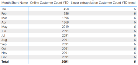
Hold on: We must always get the last month with sales. As it is now, we always get the same month as the Month of the current row.
This is because each row has the Filter Context set to each month.
Therefore, we must remove the Filter for the Month, while retaining the Year. We can do this with ALLEXCEPT():
Linear extrapolation Customer Count YTD trend =
// Get the number of months since the start of the year
VAR LastMonthWithData = CALCULATE(MAXX('Online Sales'
,RELATED('Date'[Month])
)
,ALLEXCEPT('Date', 'Date'[Year])
)

RETURN
LastMonthWithData
Now, the result looks much better:
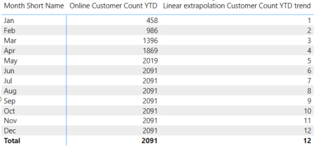
As we calculate the result for each month, we must know the month number of the current row (Month). We will reuse this as the factor for which we multiply the Average to get the linear extrapolation.
The next intermediary result is to get the Month number:
Linear extrapolation Customer Count YTD trend =
// Get the number of months since the start of the year
VAR LastMonthWithData = CALCULATE(MAXX('Online Sales'
,RELATED('Date'[Month])
)
,ALLEXCEPT('Date', 'Date'[Year])
)
// Get the last month
// Is needed if we are looking at the data at the year, semester, or
quarter level
VAR MaxMonth = MAX('Date'[Month])
RETURN
MaxMonth
I can leave the first Variable in place and only use the MaxMonth variable after the return. The result shows the month number per month:
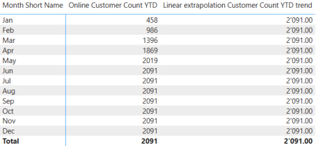
According to the definition formulated before, we must get the last Customer Count YTD for the latest month with Sales.
I can do this with the following Expression:
Linear extrapolation Customer Count YTD trend =
// Get the number of months since the start of the year
VAR LastMonthWithData = CALCULATE(MAXX('Online Sales'
,RELATED('Date'[Month])
)
,ALLEXCEPT('Date', 'Date'[Year])
)
// Get the last month
// Is needed if we are looking at the data at the year, semester, or
quarter level
VAR MaxMonth = MAX('Date'[Month])
// Get the Customer Count YTD
VAR LastCustomerCountYTD = CALCULATE([Online Customer Count YTD]
,ALLEXCEPT('Date', 'Date'[Year])
,'Date'[Month] = LastMonthWithData
)

RETURN
LastCustomerCountYTD
As expected, the result shows 2,091 for each month:
You can see why I start with a table or a Matrix when developing complex Measures.
Now, imagine that one intermediary result is a date or a text.
Showing such a result in a line visual will not be practical.
We are ready to calculate the final result according to the mathematical definition above.
Step 3: The final result
We have two ways to calculate the result:
1. Write the expression after the RETURN statement.
2. Create a new Variable “Result” and use this Variable after the RETURN statement. The final Expression is this:
(LastCustomerCountYTD / LastMonthWithData) * MaxMonthThe first Variant looks like this:
Linear extrapolation Customer Count YTD trend =
// Get the number of months since the start of the year
VAR LastMonthWithData = CALCULATE(MAXX('Online Sales'
,RELATED('Date'[Month])

)

,ALLEXCEPT('Date', 'Date'[Year])

)
// Get the last month
// Is needed if we are looking at the data at the year, semester, or
quarter level
VAR MaxMonth = MAX('Date'[Month])
// Get the Customer Count YTD
VAR LastCustomerCountYTD = CALCULATE([Online Customer Count YTD]
,ALLEXCEPT('Date', 'Date'[Year])
,'Date'[Month] = LastMonthWithData
)

RETURN
// Calculating the extrapolation
(LastCustomerCountYTD / LastMonthWithData) * MaxMonth
This is the second Variant:
Linear extrapolation Customer Count YTD trend =
// Get the number of months since the start of the year
VAR LastMonthWithData = CALCULATE(MAXX('Online Sales'
,RELATED('Date'[Month])
)
,ALLEXCEPT('Date', 'Date'[Year])
)
// Get the last month
// Is needed if we are looking at the data at the year, semester, or
quarter level
VAR MaxMonth = MAX('Date'[Month])
// Get the Customer Count YTD
VAR LastCustomerCountYTD = CALCULATE([Online Customer Count YTD]
,ALLEXCEPT('Date', 'Date'[Year])
,'Date'[Month] = LastMonthWithData
)
// Calculating the extrapolation
VAR Result =
(LastCustomerCountYTD / LastMonthWithData) * MaxMonth
RETURN
Result
The result is the same.
The second variant allows us to quickly switch back to the Intermediary results if the final result is incorrect without needing to set the expression after the RETURN statement as a comment.
It simply makes life easier.
But it’s up to you which variant you like more.
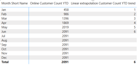
The result is this:
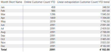
When converting this table to a Line Visual, we get the same result as in the first figure. The last step will be to set the line as a Dashed line, to get the needed visualization.
Complex calculated columns
The process is the same when writing complex DAX expressions for calculated columns. The difference is that we can see the result in the Table View of Power BI Desktop.
Be aware that when calculated columns are calculated, the results are physically stored in the table when you press Enter.
The results of Measures are not stored in the Model. They are calculated on the fly in the Visualizations.
Another difference is that we can leverage Context Transition to get our result when we need it to depend on other rows in the table.
Read this piece to learn more about this fascinating topic:
Conclusion
The development process for complex expressions always follows the same steps:
1. Understand the requirements – Ask if something is unclear.
2. Define the math for the results.
3. Start with intermediary results and understand the results.
4. Build on the intermediary results one by one – Do not try to write all in one step.
5. Decide where to write the expression for the final result.
Following such a process can save you the day, as you don’t need to write everything in one step.
Moreover, getting these intermediary results allows you to understand what’s happening and explore the Filter Context.
This will help you learn DAX more efficiently and build even more complex stuff.
But, be aware: Even though a certain level of complexity is needed, a good developer will keep it as simple as possible, while maintaining the least amount of complexity.
References
Here is the article mentioned at the beginning of this piece, to calculate the linear interpolation.
Like in my previous articles, I use the Contoso sample dataset. You can download the ContosoRetailDW Dataset for free from Microsoft here.
The Contoso Data can be freely used under the MIT License, as described here. I changed the dataset to shift the data to contemporary dates.