In today’s world, the reliability of data solutions is everything. When we build dashboards and reports, one expects that the numbers reflected there are correct and up-to-date. Based on these numbers, insights are drawn and actions are taken. For any unforeseen reason, if the dashboards are broken or if the numbers are incorrect — then it becomes a fire-fight to fix everything. If the issues are not fixed in time, then it damages the trust placed on the data team and their solutions.
But why would dashboards be broken or have wrong numbers? If the dashboard was built correctly the first time, then 99% of the time the issue comes from the data that feeds the dashboards — from the data warehouse. Some possible scenarios are:
- Few ETL pipelines failed, so the new data is not yet in
- A table is replaced with another new one
- Some columns in the table are dropped or renamed
- Schemas in data warehouse have changed
- And many more.
There is still a chance that the issue is on the Tableau site, but in my experience, most of the times, it is always due to some changes in data warehouse. Even though we know the root cause, it’s not always straightforward to start working on a fix. There is no central place where you can check which Tableau data sources rely on specific tables. If you have the Tableau Data Management add-on, it could help, but from what I know, its hard to find dependencies of custom sql queries used in data sources.
Nevertheless, the add-on is too expensive and most companies don’t have it. The real pain begins when you have to go through all the data sources manually to start fixing it. On top of it, you have a string of users on your head impatiently waiting for a quick-fix. The fix itself might not be difficult, it would just be a time-consuming one.
What if we could anticipate these issues and identify impacted data sources before anyone notices a problem? Wouldn’t that just be great? Well, there is a way now with the Tableau Metadata API. The Metadata API uses GraphQL, a query language for APIs that returns only the data that you’re interested in. For more info on what’s possible with GraphQL, do check out GraphQL.org.
In this blog post, I’ll show you how to connect to the Tableau Metadata API using Python’s Tableau Server Client (TSC) library to proactively identify data sources using specific tables, so that you can act fast before any issues arise. Once you know which Tableau data sources are affected by a specific table, you can make some updates yourself or alert the owners of those data sources about the upcoming changes so they can be prepared for it.
Connecting to the Tableau Metadata API
Lets connect to the Tableau Server using TSC. We need to import in all the libraries we would need for the exercise!
### Import all required libraries
import tableauserverclient as t
import pandas as pd
import json
import ast
import re
In order to connect to the Metadata API, you will have to first create a personal access token in your Tableau Account settings. Then update the & with the token you just created. Also update with your Tableau site. If the connection is established successfully, then “Connected” will be printed in the output window.
### Connect to Tableau server using personal access token
tableau_auth = t.PersonalAccessTokenAuth("", "",
                                           site_id="")
server = t.Server("https://dub01.online.tableau.com/", use_server_version=True)

with server.auth.sign_in(tableau_auth):
        print("Connected")
Lets now get a list of all data sources that are published on your site. There are many attributes you can fetch, but for the current use case, lets keep it simple and only get the id, name and owner contact information for every data source. This will be our master list to which we will add in all other information.
############### Get all the list of data sources on your Site

all_datasources_query = """ {
  publishedDatasources {
    name
    id
    owner {
    name
    email
    }
  }
}"""
with server.auth.sign_in(tableau_auth):
    result = server.metadata.query(
        all_datasources_query
    )
Since I want this blog to be focussed on how to proactively identify which data sources are affected by a specific table, I’ll not be going into the nuances of Metadata API. To better understand how the query works, you can refer to a very detailed Tableau’s own Metadata API documentation.
One thing to note is that the Metadata API returns data in a JSON format. Depending on what you are querying, you’ll end up with multiple nested json lists and it can get very tricky to convert this into a pandas dataframe. For the above metadata query, you will end up with a result which would like below (this is mock data just to give you an idea of what the output looks like):
{
"data": {
"publishedDatasources": [
{
"name": "Sales Performance DataSource",
"id": "f3b1a2c4-1234-5678-9abc-1234567890ab",
"owner": {
"name": "Alice Johnson",
"email": "[email protected]"
}
},
{
"name": "Customer Orders DataSource",
"id": "a4d2b3c5-2345-6789-abcd-2345678901bc",
"owner": {
"name": "Bob Smith",
"email": "[email protected]"
}
},
{
"name": "Product Returns and Profitability",
"id": "c5e3d4f6-3456-789a-bcde-3456789012cd",
"owner": {
"name": "Alice Johnson",
"email": "[email protected]"
}
},
{
"name": "Customer Segmentation Analysis",
"id": "d6f4e5a7-4567-89ab-cdef-4567890123de",
"owner": {
"name": "Charlie Lee",
"email": "[email protected]"
}
},
{
"name": "Regional Sales Trends (Custom SQL)",
"id": "e7a5f6b8-5678-9abc-def0-5678901234ef",
"owner": {
"name": "Bob Smith",
"email": "[email protected]"
}
}
]
}
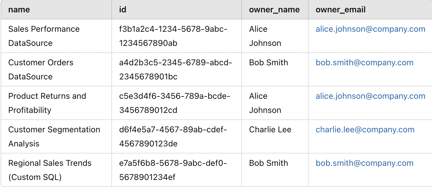
}We need to convert this JSON response into a dataframe so that its easy to work with. Notice that we need to extract the name and email of the owner from inside the owner object.
### We need to convert the response into dataframe for easy data manipulation

col_names = result['data']['publishedDatasources'][0].keys()
master_df = pd.DataFrame(columns=col_names)

for i in result['data']['publishedDatasources']:
    tmp_dt = {k:v for k,v in i.items()}
    master_df = pd.concat([master_df, pd.DataFrame.from_dict(tmp_dt, orient='index').T])

# Extract the owner name and email from the owner object
master_df['owner_name'] = master_df['owner'].apply(lambda x: x.get('name') if isinstance(x, dict) else None)
master_df['owner_email'] = master_df['owner'].apply(lambda x: x.get('email') if isinstance(x, dict) else None)

master_df.reset_index(inplace=True)
master_df.drop(['index','owner'], axis=1, inplace=True)
print('There are ', master_df.shape[0] , ' datasources in your site')
This is how the structure of master_df would look like:
Once we have the main list ready, we can go ahead and start getting the names of the tables embedded in the data sources. If you are an avid Tableau user, you know that there are two ways to selecting tables in a Tableau data source — one is to directly choose the tables and establish a relation between them and the other is to use a custom sql query with one or more tables to achieve a new resultant table. Therefore, we need to address both the cases.
Processing of Custom SQL query tables
Below is the query to get the list of all custom SQLs used in the site along with their data sources. Notice that I have filtered the list to get only first 500 custom sql queries. In case there are more in your org, you will have to use an offset to get the next set of custom sql queries. There is also an option of using cursor method in Pagination when you want to fetch large list of results (refer here). For the sake of simplicity, I just use the offset method as I know, as there are less than 500 custom sql queries used on the site.
# Get the data sources and the table names from all the custom sql queries used on your Site

custom_table_query = """  {
  customSQLTablesConnection(first: 500){
    nodes {
        id
        name
        downstreamDatasources {
        name
        }
        query
    }
  }
}
"""

with server.auth.sign_in(tableau_auth):
    custom_table_query_result = server.metadata.query(
        custom_table_query
    )
Based on our mock data, this is how our output would look like:
{
"data": {
"customSQLTablesConnection": {
"nodes": [
{
"id": "csql-1234",
"name": "RegionalSales_CustomSQL",
"downstreamDatasources": [
{
"name": "Regional Sales Trends (Custom SQL)"
}
],
"query": "SELECT r.region_name, SUM(s.sales_amount) AS total_sales FROM ecommerce.sales_data.Sales s JOIN ecommerce.sales_data.Regions r ON s.region_id = r.region_id GROUP BY r.region_name"
},
{
"id": "csql-5678",
"name": "ProfitabilityAnalysis_CustomSQL",
"downstreamDatasources": [
{
"name": "Product Returns and Profitability"
}
],
"query": "SELECT p.product_category, SUM(s.profit) AS total_profit FROM ecommerce.sales_data.Sales s JOIN ecommerce.sales_data.Products p ON s.product_id = p.product_id GROUP BY p.product_category"
},
{
"id": "csql-9101",
"name": "CustomerSegmentation_CustomSQL",
"downstreamDatasources": [
{
"name": "Customer Segmentation Analysis"
}
],
"query": "SELECT c.customer_id, c.location, COUNT(o.order_id) AS total_orders FROM ecommerce.sales_data.Customers c JOIN ecommerce.sales_data.Orders o ON c.customer_id = o.customer_id GROUP BY c.customer_id, c.location"
},
{
"id": "csql-3141",
"name": "CustomerOrders_CustomSQL",
"downstreamDatasources": [
{
"name": "Customer Orders DataSource"
}
],
"query": "SELECT o.order_id, o.customer_id, o.order_date, o.sales_amount FROM ecommerce.sales_data.Orders o WHERE o.order_status = 'Completed'"
},
{
"id": "csql-3142",
"name": "CustomerProfiles_CustomSQL",
"downstreamDatasources": [
{
"name": "Customer Orders DataSource"
}
],
"query": "SELECT c.customer_id, c.customer_name, c.segment, c.location FROM ecommerce.sales_data.Customers c WHERE c.active_flag = 1"
},
{
"id": "csql-3143",
"name": "CustomerReturns_CustomSQL",
"downstreamDatasources": [
{
"name": "Customer Orders DataSource"
}
],
"query": "SELECT r.return_id, r.order_id, r.return_reason FROM ecommerce.sales_data.Returns r"
}
]
}
}
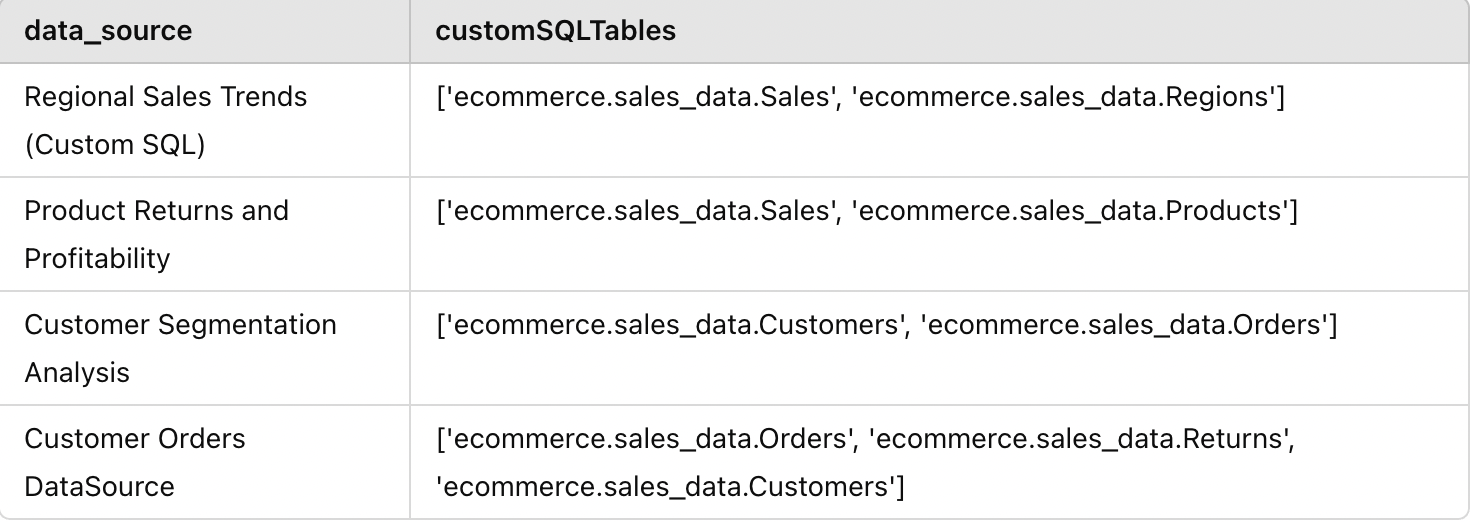
}Just like before when we were creating the master list of data sources, here also we have nested json for the downstream data sources where we would need to extract only the “name” part of it. In the “query” column, the entire custom sql is dumped. If we use regex pattern, we can easily search for the names of the table used in the query.
We know that the table names always come after FROM or a JOIN clause and they generally follow the format ..
. The is optional and most of the times not used. There were some queries I found which used this format and I ended up only getting the database and schema names, and not the complete table name. Once we have extracted the names of the data sources and the names of the tables, we need to merge the rows per data source as there can be multiple custom sql queries used in a single data source.
### Convert the custom sql response into dataframe
col_names = custom_table_query_result['data']['customSQLTablesConnection']['nodes'][0].keys()
cs_df = pd.DataFrame(columns=col_names)

for i in custom_table_query_result['data']['customSQLTablesConnection']['nodes']:
    tmp_dt = {k:v for k,v in i.items()}

    cs_df = pd.concat([cs_df, pd.DataFrame.from_dict(tmp_dt, orient='index').T])

# Extract the data source name where the custom sql query was used
cs_df['data_source'] = cs_df.downstreamDatasources.apply(lambda x: x[0]['name'] if x and 'name' in x[0] else None)
cs_df.reset_index(inplace=True)
cs_df.drop(['index','downstreamDatasources'], axis=1,inplace=True)

### We need to extract the table names from the sql query. We know the table name comes after FROM or JOIN clause
# Note that the name of table can be of the format ..
# Depending on the format of how table is called, you will have to modify the regex expression

def extract_tables(sql):
    # Regex to match database.schema.table or schema.table, avoid alias
    pattern = r'(?:FROM|JOIN)s+((?:[w+]|w+).(?:[w+]|w+)(?:.(?:[w+]|w+))?)b'
    matches = re.findall(pattern, sql, re.IGNORECASE)
    return list(set(matches))  # Unique table names

cs_df['customSQLTables'] = cs_df['query'].apply(extract_tables)
cs_df = cs_df[['data_source','customSQLTables']]

# We need to merge datasources as there can be multiple custom sqls used in the same data source
cs_df = cs_df.groupby('data_source', as_index=False).agg({
    'customSQLTables': lambda x: list(set(item for sublist in x for item in sublist))  # Flatten & make unique
})

print('There are ', cs_df.shape[0], 'datasources with custom sqls used in it')
After we perform all the above operations, this is how the structure of cs_df would look like:
Processing of regular Tables in Data Sources
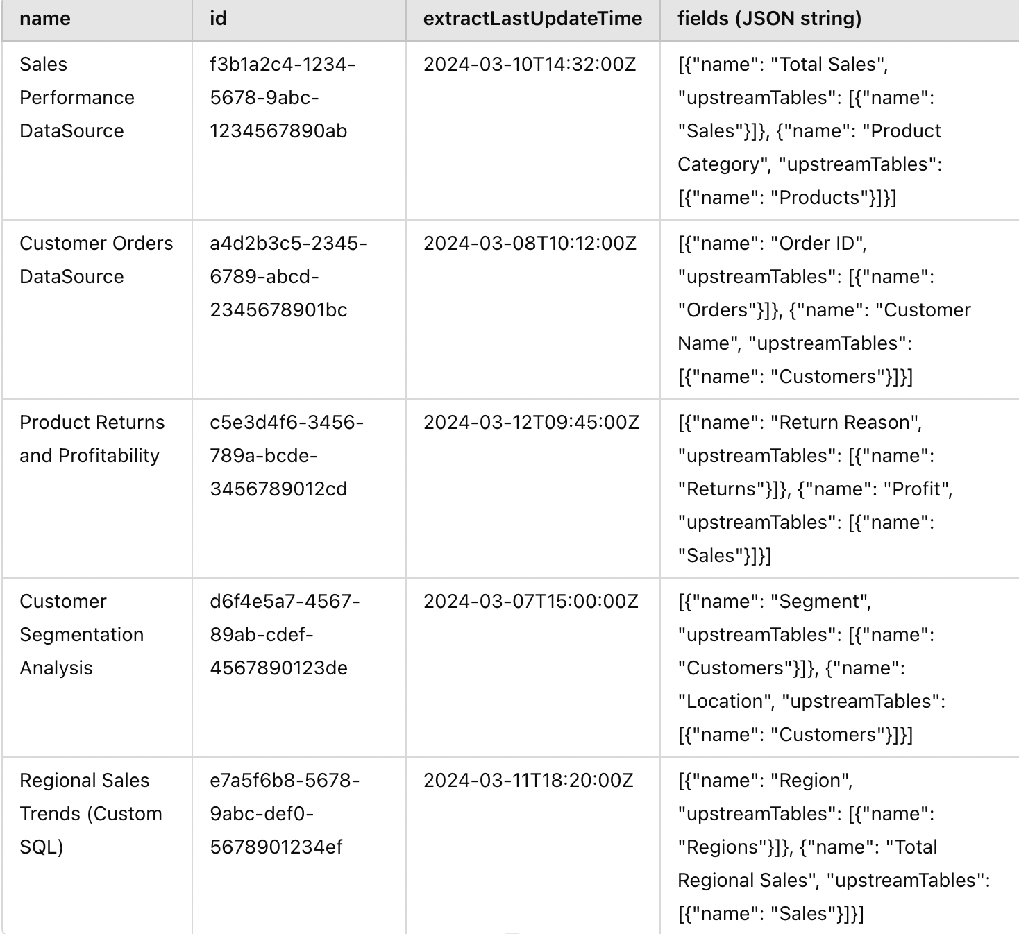
Now we need to get the list of all the regular tables used in a datasource which are not a part of custom SQL. There are two ways to go about it. Either use the publishedDatasources object and check for upstreamTables or use DatabaseTable and check for upstreamDatasources. I’ll go by the first method because I want the results at a data source level (basically, I want some code ready to reuse when I want to check a specific data source in further detail). Here again, for the sake of simplicity, instead of going for pagination, I’m looping through each datasource to ensure I have everything. We get the upstreamTables inside of the field object so that has to be cleaned out.
############### Get the data sources with the regular table names used in your site

### Its best to extract the tables information for every data source and then merge the results.
# Since we only get the table information nested under fields, in case there are hundreds of fields
# used in a single data source, we will hit the response limits and will not be able to retrieve all the data.

data_source_list = master_df.name.tolist()

col_names = ['name', 'id', 'extractLastUpdateTime', 'fields']
ds_df = pd.DataFrame(columns=col_names)

with server.auth.sign_in(tableau_auth):
    for ds_name in data_source_list:
        query = """ {
            publishedDatasources (filter: { name: """"+ ds_name + """" }) {
            name
            id
            extractLastUpdateTime
            fields {
                name
                upstreamTables {
                    name
                }
            }
            }
        } """
        ds_name_result = server.metadata.query(
        query
        )
        for i in ds_name_result['data']['publishedDatasources']:
            tmp_dt = {k:v for k,v in i.items() if k != 'fields'}
            tmp_dt['fields'] = json.dumps(i['fields'])
        ds_df = pd.concat([ds_df, pd.DataFrame.from_dict(tmp_dt, orient='index').T])

ds_df.reset_index(inplace=True)
This is how the structure of ds_df would look:
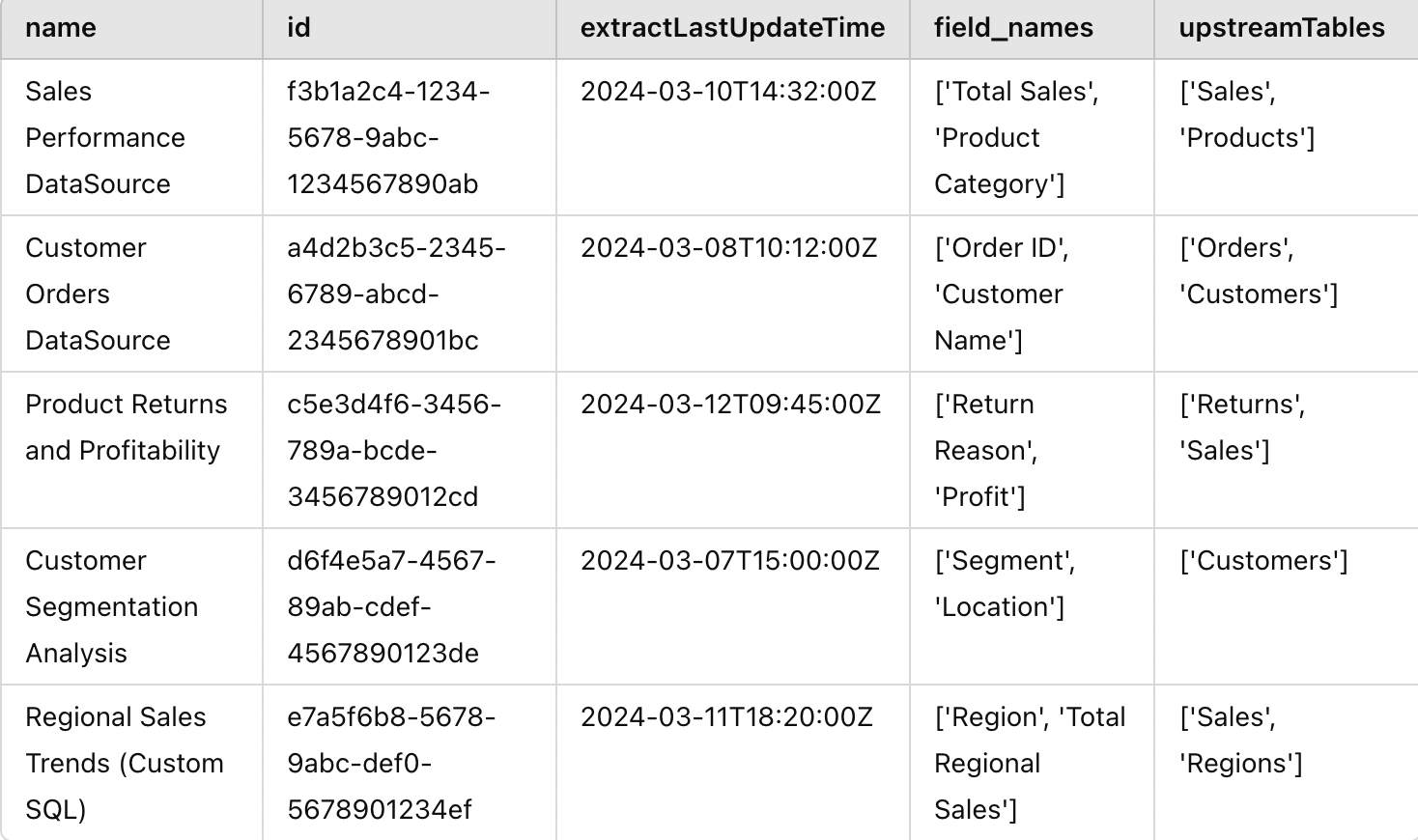
We can need to flatten out the fields object and extract the field names as well as the table names. Since the table names will be repeating multiple times, we would have to deduplicate to keep only the unique ones.
# Function to extract the values of fields and upstream tables in json lists
def extract_values(json_list, key):
    values = []
    for item in json_list:
        values.append(item[key])
    return values

ds_df["fields"] = ds_df["fields"].apply(ast.literal_eval)
ds_df['field_names'] = ds_df.apply(lambda x: extract_values(x['fields'],'name'), axis=1)
ds_df['upstreamTables'] = ds_df.apply(lambda x: extract_values(x['fields'],'upstreamTables'), axis=1)

# Function to extract the unique table names
def extract_upstreamTable_values(table_list):
    values = set()a
    for inner_list in table_list:
        for item in inner_list:
            if 'name' in item:
                values.add(item['name'])
    return list(values)

ds_df['upstreamTables'] = ds_df.apply(lambda x: extract_upstreamTable_values(x['upstreamTables']), axis=1)
ds_df.drop(["index","fields"], axis=1, inplace=True)
Once we do the above operations, the final structure of ds_df would look something like this:
We have all the pieces and now we just have to merge them together:
###### Join all the data together
master_data = pd.merge(master_df, ds_df, how="left", on=["name","id"])
master_data = pd.merge(master_data, cs_df, how="left", left_on="name", right_on="data_source")
# Save the results to analyse further
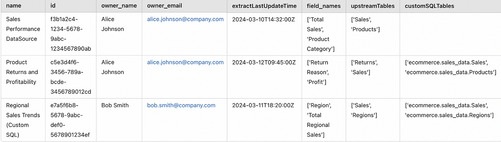
master_data.to_excel("Tableau Data Sources with Tables.xlsx", index=False)This is our final master_data:
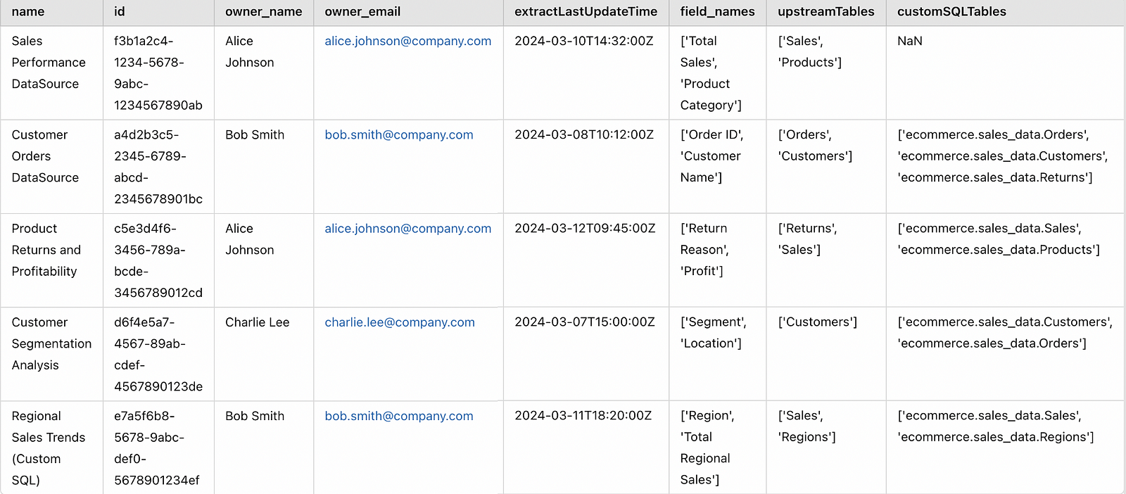
Table-level Impact Analysis
Let’s say there were some schema changes on the “Sales” table and you want to know which data sources will be impacted. Then you can simply write a small function which checks if a table is present in either of the two columns — upstreamTables or customSQLTables like below.
def filter_rows_with_table(df, col1, col2, target_table):
    """
    Filters rows in df where target_table is part of any value in either col1 or col2 (supports partial match).
    Returns full rows (all columns retained).
    """
    return df[
        df.apply(
            lambda row:
                (isinstance(row[col1], list) and any(target_table in item for item in row[col1])) or
                (isinstance(row[col2], list) and any(target_table in item for item in row[col2])),
            axis=1
        )
    ]
# As an example
filter_rows_with_table(master_data, 'upstreamTables', 'customSQLTables', 'Sales')
Below is the output. You can see that 3 data sources will be impacted by this change. You can also alert the data source owners Alice and Bob in advance about this so they can start working on a fix before something breaks on the Tableau dashboards.
You can check out the complete version of the code in my Github repository here.
This is just one of the potential use-cases of the Tableau Metadata API. You can also extract the field names used in custom sql queries and add to the dataset to get a field-level impact analysis. One can also monitor the stale data sources with the extractLastUpdateTime to see if those have any issues or need to be archived if they are not used any more. We can also use the dashboards object to fetch information at a dashboard level.
Final Thoughts
If you have come this far, kudos. This is just one use case of automating Tableau data management. It’s time to reflect on your own work and think which of those other tasks you could automate to make your life easier. I hope this mini-project served as an enjoyable learning experience to understand the power of Tableau Metadata API. If you liked reading this, you might also like another one of my blog posts about Tableau, on some of the challenges I faced when dealing with big .
Also do check out my previous blog where I explored building an interactive, database-powered app with Python, Streamlit, and SQLite.
Before you go…
Follow me so you don’t miss any new posts I write in future; you will find more of my articles on my . You can also connect with me on LinkedIn or Twitter!