There are some Sql patterns that, once you know them, you start seeing them everywhere. The solutions to the puzzles that I will show you today are actually very simple SQL queries, but understanding the concept behind them will surely unlock new solutions to the queries you write on a day-to-day basis.
These challenges are all based on real-world scenarios, as over the past few months I made a point of writing down every puzzle-like query that I had to build. I also encourage you to try them for yourself, so that you can challenge yourself first, which will improve your learning!
All queries to generate the datasets will be provided in a PostgreSQL and DuckDB-friendly syntax, so that you can easily copy and play with them. At the end I will also provide you a link to a GitHub repo containing all the code, as well as the answer to the bonus challenge I will leave for you!
I organized these puzzles in order of increasing difficulty, so, if you find the first ones too easy, at least take a look at the last one, which uses a technique that I truly believe you won’t have seen before.
Okay, let’s get started.
I love this puzzle because of how short and simple the final query is, even though it deals with many edge cases. The data for this challenge shows tickets moving in between Kanban stages, and the objective is to find how long, on average, tickets stay in the Doing stage.
The data contains the ID of the ticket, the date the ticket was created, the date of the move, and the “from” and “to” stages of the move. The stages present are New, Doing, Review, and Done.
Some things you need to know (edge cases):
- Tickets can move backwards, meaning tickets can go back to the Doing stage.
- You should not include tickets that are still stuck in the Doing stage, as there is no way to know how long they will stay there for.
- Tickets are not always created in the New stage.
```SQL

CREATE TABLE ticket_moves (
    ticket_id INT NOT NULL,
    create_date DATE NOT NULL,
    move_date DATE NOT NULL,
    from_stage TEXT NOT NULL,
    to_stage TEXT NOT NULL
);

```
```SQL
INSERT INTO ticket_moves (ticket_id, create_date, move_date, from_stage, to_stage)
VALUES
-- Ticket 1: Created in "New", then moves to Doing, Review, Done.
(1, '2024-09-01', '2024-09-03', 'New', 'Doing'),
(1, '2024-09-01', '2024-09-07', 'Doing', 'Review'),
(1, '2024-09-01', '2024-09-10', 'Review', 'Done'),
-- Ticket 2: Created in "New", then moves: New → Doing → Review → Doing again → Review.
(2, '2024-09-05', '2024-09-08', 'New', 'Doing'),
(2, '2024-09-05', '2024-09-12', 'Doing', 'Review'),
(2, '2024-09-05', '2024-09-15', 'Review', 'Doing'),
(2, '2024-09-05', '2024-09-20', 'Doing', 'Review'),
-- Ticket 3: Created in "New", then moves to Doing. (Edge case: no subsequent move from Doing.)
(3, '2024-09-10', '2024-09-16', 'New', 'Doing'),
-- Ticket 4: Created already in "Doing", then moves to Review.
(4, '2024-09-15', '2024-09-22', 'Doing', 'Review');
```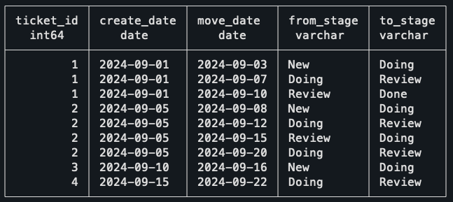
A summary of the data:
- Ticket 1: Created in the New stage, moves normally to Doing, then Review, and then Done.
- Ticket 2: Created in New, then moves: New → Doing → Review → Doing again → Review.
- Ticket 3: Created in New, moves to Doing, but it is still stuck there.
- Ticket 4: Created in the Doing stage, moves to Review afterward.
It might be a good idea to stop for a bit and think how you would deal with this. Can you find out how long a ticket stays on a single stage?
Honestly, this sounds intimidating at first, and it looks like it will be a nightmare to deal with all the edge cases. Let me show you the full solution to the problem, and then I will explain what is happening afterward.
```SQL

WITH stage_intervals AS (
    SELECT
        ticket_id,
        from_stage,
        move_date
        - COALESCE(
            LAG(move_date) OVER (
                PARTITION BY ticket_id
                ORDER BY move_date
            ),
            create_date
        ) AS days_in_stage
    FROM
        ticket_moves
)
SELECT
    SUM(days_in_stage) / COUNT(DISTINCT ticket_id) as avg_days_in_doing
FROM
    stage_intervals
WHERE
    from_stage = 'Doing';
```
The first CTE uses the LAG function to find the previous move of the ticket, which will be the time the ticket entered that stage. Calculating the duration is as simple as subtracting the previous date from the move date.
What you should notice is the use of the COALESCE in the previous move date. What that does is that if a ticket doesn’t have a previous move, then it uses the date of creation of the ticket. This takes care of the cases of tickets being created directly into the Doing stage, as it still will properly calculate the time it took to leave the stage.
This is the result of the first CTE, showing the time spent in each stage. Notice how the Ticket 2 has two entries, as it visited the Doing stage in two separate occasions.
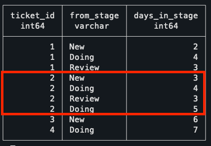
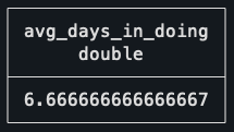
With this done, it’s just a matter of getting the average as the SUM of total days spent in doing, divided by the distinct number of tickets that ever left the stage. Doing it this way, instead of simply using the AVG, makes sure that the two rows for Ticket 2 get properly accounted for as a single ticket.
Not so bad, right?
The goal of this second challenge is to find the most recent contract sequence of every employee. A break of sequence happens when two contracts have a gap of more than one day between them.
In this dataset, there are no contract overlaps, meaning that a contract for the same employee either has a gap or ends a day before the new one starts.
```SQL
CREATE TABLE contracts (
    contract_id integer PRIMARY KEY,
    employee_id integer NOT NULL,
    start_date date NOT NULL,
    end_date date NOT NULL
);

INSERT INTO contracts (contract_id, employee_id, start_date, end_date)
VALUES
    -- Employee 1: Two continuous contracts
    (1, 1, '2024-01-01', '2024-03-31'),
    (2, 1, '2024-04-01', '2024-06-30'),
    -- Employee 2: One contract, then a gap of three days, then two contracts
    (3, 2, '2024-01-01', '2024-02-15'),
    (4, 2, '2024-02-19', '2024-04-30'),
    (5, 2, '2024-05-01', '2024-07-31'),
    -- Employee 3: One contract
    (6, 3, '2024-03-01', '2024-08-31');
```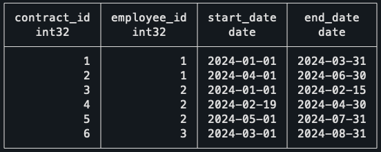
As a summary of the data:
- Employee 1: Has two continuous contracts.
- Employee 2: One contract, then a gap of three days, then two contracts.
- Employee 3: One contract.
The expected result, given the dataset, is that all contracts should be included except for the first contract of Employee 2, which is the only one that has a gap.
Before explaining the logic behind the solution, I would like you to think about what operation can be used to join the contracts that belong to the same sequence. Focus only on the second row of data, what information do you need to know if this contract was a break or not?
I hope it’s clear that this is the perfect situation for window functions, again. They are incredibly useful for solving problems like this, and understanding when to use them helps a lot in finding clean solutions to problems.
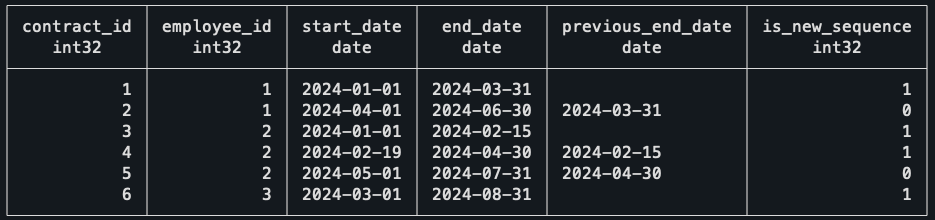
First thing to do, then, is to get the end date of the previous contract for the same employee with the LAG function. Doing that, it’s simple to compare both dates and check if it was a break of sequence.
```SQL
WITH ordered_contracts AS (
    SELECT
        *,
        LAG(end_date) OVER (PARTITION BY employee_id ORDER BY start_date) AS previous_end_date
    FROM
        contracts
),
gapped_contracts AS (
    SELECT
        *,
        -- Deals with the case of the first contract, which won't have
        -- a previous end date. In this case, it's still the start of a new
        -- sequence.
        CASE WHEN previous_end_date IS NULL
            OR previous_end_date < start_date - INTERVAL '1 day' THEN
            1
        ELSE
            0
        END AS is_new_sequence
    FROM
        ordered_contracts
)
SELECT * FROM gapped_contracts ORDER BY employee_id ASC;
```
An intuitive way to continue the query is to number the sequences of each employee. For example, an employee who has no gap, will always be on his first sequence, but an employee who had 5 breaks in contracts will be on his 5th sequence. Funnily enough, this is done by another window function.
```SQL
--
-- Previous CTEs
--
sequences AS (
    SELECT
        *,
        SUM(is_new_sequence) OVER (PARTITION BY employee_id ORDER BY start_date) AS sequence_id
FROM
    gapped_contracts
)
SELECT * FROM sequences ORDER BY employee_id ASC;
```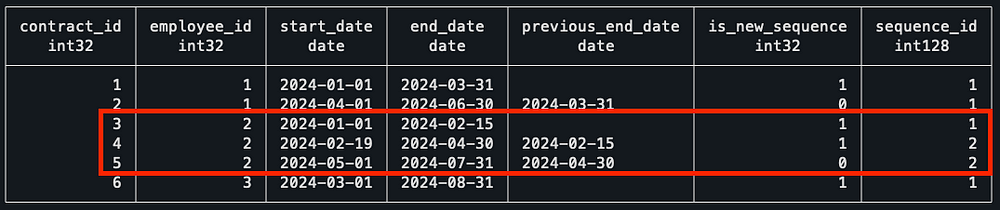
Notice how, for Employee 2, he starts his sequence #2 after the first gapped value. To finish this query, I grouped the data by employee, got the value of their most recent sequence, and then did an inner join with the sequences to keep only the most recent one.
```SQL
--
-- Previous CTEs
--
max_sequence AS (
    SELECT
        employee_id,
        MAX(sequence_id) AS max_sequence_id
FROM
    sequences
GROUP BY
    employee_id
),
latest_contract_sequence AS (
    SELECT
        c.contract_id,
        c.employee_id,
        c.start_date,
        c.end_date
    FROM
        sequences c
        JOIN max_sequence m ON c.sequence_id = m.max_sequence_id
            AND c.employee_id = m.employee_id
        ORDER BY
            c.employee_id,
            c.start_date
)
SELECT
    *
FROM
    latest_contract_sequence;
```
As expected, our final result is basically our starting query just with the first contract of Employee 2 missing!
Finally, the last puzzle — I’m glad you made it this far.
For me, this is the most mind-blowing one, as when I first encountered this problem I thought of a completely different solution that would be a mess to implement in SQL.
For this puzzle, I’ve changed the context from what I had to deal with for my job, as I think it will make it easier to explain.
Imagine you’re a data analyst at an event venue, and you’re analyzing the talks scheduled for an upcoming event. You want to find the time of day where there will be the highest number of talks happening at the same time.
This is what you should know about the schedules:
- Rooms are booked in increments of 30min, e.g. from 9h-10h30.
- The data is clean, there are no overbookings of meeting rooms.
- There can be back-to-back meetings in a single meeting room.
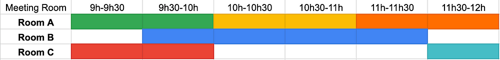
Meeting schedule visualized (this is the actual data).
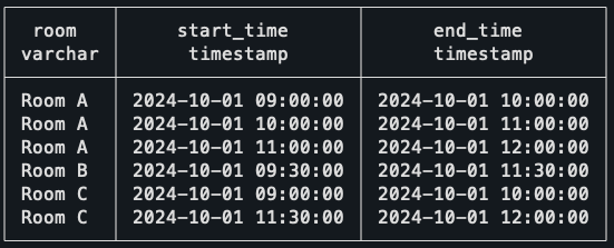
```SQL
CREATE TABLE meetings (
    room TEXT NOT NULL,
    start_time TIMESTAMP NOT NULL,
    end_time TIMESTAMP NOT NULL
);

INSERT INTO meetings (room, start_time, end_time) VALUES
    -- Room A meetings
    ('Room A', '2024-10-01 09:00', '2024-10-01 10:00'),
    ('Room A', '2024-10-01 10:00', '2024-10-01 11:00'),
    ('Room A', '2024-10-01 11:00', '2024-10-01 12:00'),
    -- Room B meetings
    ('Room B', '2024-10-01 09:30', '2024-10-01 11:30'),
    -- Room C meetings
    ('Room C', '2024-10-01 09:00', '2024-10-01 10:00'),
    ('Room C', '2024-10-01 11:30', '2024-10-01 12:00');
```
The way to solve this is using what is called a Sweep Line Algorithm, or also known as an event-based solution. This last name actually helps to understand what will be done, as the idea is that instead of dealing with intervals, which is what we have in the original data, we deal with events instead.
To do this, we need to transform every row into two separate events. The first event will be the Start of the meeting, and the second event will be the End of the meeting.
```SQL
WITH events AS (
  -- Create an event for the start of each meeting (+1)
  SELECT
    start_time AS event_time,
    1 AS delta
  FROM meetings
  UNION ALL
  -- Create an event for the end of each meeting (-1)
  SELECT
   -- Small trick to work with the back-to-back meetings (explained later)
    end_time - interval '1 minute' as end_time,
    -1 AS delta
  FROM meetings
)
SELECT * FROM events;
```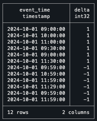
Take the time to understand what is happening here. To create two events from a single row of data, we’re simply unioning the dataset on itself; the first half uses the start time as the timestamp, and the second part uses the end time.
You might already notice the delta column created and see where this is going. When an event starts, we count it as +1, when it ends, we count it as -1. You might even be already thinking of another window function to solve this, and you’re actually right!
But before that, let me just explain the trick I used in the end dates. As I don’t want back-to-back meetings to count as two concurrent meetings, I’m subtracting a single minute of every end date. This way, if a meeting ends and another starts at 10h30, it won’t be assumed that two meetings are concurrently happening at 10h30.
Okay, back to the query and yet another window function. This time, though, the function of choice is a rolling SUM.
```SQL
--
-- Previous CTEs
--
ordered_events AS (
  SELECT
    event_time,
    delta,
    SUM(delta) OVER (ORDER BY event_time, delta DESC) AS concurrent_meetings
  FROM events
)
SELECT * FROM ordered_events ORDER BY event_time DESC;
```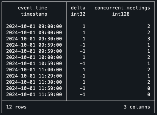
The rolling SUM at the Delta column is essentially walking down every record and finding how many events are active at that time. For example, at 9 am sharp, it sees two events starting, so it marks the number of concurrent meetings as two!
When the third meeting starts, the count goes up to three. But when it gets to 9h59 (10 am), then two meetings end, bringing the counter back to one. With this data, the only thing missing is to find when the highest value of concurrent meetings happens.
```SQL
--
-- Previous CTEs
--
max_events AS (
  -- Find the maximum concurrent meetings value
  SELECT
    event_time,
    concurrent_meetings,
    RANK() OVER (ORDER BY concurrent_meetings DESC) AS rnk
  FROM ordered_events
)
SELECT event_time, concurrent_meetings
FROM max_events
WHERE rnk = 1;
```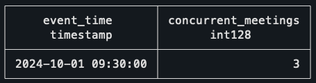
That’s it! The interval of 9h30–10h is the one with the largest number of concurrent meetings, which checks out with the schedule visualization above!
This solution looks incredibly simple in my opinion, and it works for so many situations. Every time you are dealing with intervals now, you should think if the query wouldn’t be easier if you thought about it in the perspective of events.
But before you move on, and to really nail down this concept, I want to leave you with a bonus challenge, which is also a common application of the Sweep Line Algorithm. I hope you give it a try!
Bonus challenge
The context for this one is still the same as the last puzzle, but now, instead of trying to find the period when there are most concurrent meetings, the objective is to find bad scheduling. It seems that there are overlaps in the meeting rooms, which need to be listed so it can be fixed ASAP.
How would you find out if the same meeting room has two or more meetings booked at the same time? Here are some tips on how to solve it:
- It’s still the same algorithm.
- This means you will still do the UNION, but it will look slightly different.
- You should think in the perspective of each meeting room.
You can use this data for the challenge:
```SQL
CREATE TABLE meetings_overlap (
    room TEXT NOT NULL,
    start_time TIMESTAMP NOT NULL,
    end_time TIMESTAMP NOT NULL
);

INSERT INTO meetings_overlap (room, start_time, end_time) VALUES
    -- Room A meetings
    ('Room A', '2024-10-01 09:00', '2024-10-01 10:00'),
    ('Room A', '2024-10-01 10:00', '2024-10-01 11:00'),
    ('Room A', '2024-10-01 11:00', '2024-10-01 12:00'),
    -- Room B meetings
    ('Room B', '2024-10-01 09:30', '2024-10-01 11:30'),
    -- Room C meetings
    ('Room C', '2024-10-01 09:00', '2024-10-01 10:00'),
    -- Overlaps with previous meeting.
    ('Room C', '2024-10-01 09:30', '2024-10-01 12:00');
```
If you’re interested in the solution to this puzzle, as well as the rest of the queries, check this GitHub repo.
The first takeaway from this blog post is that window functions are overpowered. Ever since I got more comfortable with using them, I feel that my queries have gotten so much simpler and easier to read, and I hope the same happens to you.
If you’re interested in learning more about them, you would probably enjoy reading this other blog post I’ve written, where I go over how you can understand and use them effectively.
The second takeaway is that these patterns used in the challenges really do happen in many other places. You might need to find sequences of subscriptions, customer retention, or you might need to find overlap of tasks. There are many situations when you will need to use window functions in a very similar fashion to what was done in the puzzles.
The third thing I want you to remember is about this solution to using events besides dealing with intervals. I’ve looked at some problems I solved a long time ago that I could’ve used this pattern on to make my life easier, and unfortunately, I didn’t know about it at the time.
I really do hope you enjoyed this post and gave a shot to the puzzles yourself. And I’m sure that if you made it this far, you either learned something new about SQL or strengthened your knowledge of window functions!
Thank you so much for reading. If you have questions or just want to get in touch with me, don’t hesitate to contact me at mtrentz.com.
All images by the author unless stated otherwise.