With the new age of problem-solving augmented by Large Language Models (LLMs), only a handful of problems remain that have subpar solutions. Most classification problems (at a PoC level) can be solved by leveraging LLMs at 70–90% Precision/F1 with just good prompt engineering techniques, as well as adaptive in-context-learning (ICL) examples.
What happens when you want to consistently achieve performance higher than that — when prompt engineering no longer suffices?
The classification conundrum
Text classification is one of the oldest and most well-understood examples of supervised learning. Given this premise, it should really not be hard to build robust, well-performing classifiers that handle a large number of input classes, right…?
Welp. It is.
It actually has to do a lot more with the ‘constraints’ that the algorithm is generally expected to work under:
- low amount of training data per class
- high classification accuracy (that plummets as you add more classes)
- possible addition of new classes to an existing subset of classes
- quick training/inference
- cost-effectiveness
- (potentially) really large number of training classes
- (potentially) endless required retraining of some classes due to data drift, etc.
Ever tried building a classifier beyond a few dozen classes under these conditions? (I mean, even GPT could probably do a great job up to ~30 text classes with just a few samples…)
Considering you take the GPT route — If you have more than a couple dozen classes or a sizeable amount of data to be classified, you are gonna have to reach deep into your pockets with the system prompt, user prompt, few shot example tokens that you will need to classify one sample. That is after making peace with the throughput of the API, even if you are running async queries.
In applied ML, problems like these are generally tricky to solve since they don’t fully satisfy the requirements of supervised learning or aren’t cheap/fast enough to be run via an LLM. This particular pain point is what the R.E.D algorithm addresses: semi-supervised learning, when the training data per class is not enough to build (quasi)traditional classifiers.
The R.E.D. algorithm
R.E.D: Recursive Expert Delegation is a novel framework that changes how we approach text classification. This is an applied ML paradigm — i.e., there is no fundamentally different architecture to what exists, but its a highlight reel of ideas that work best to build something that is practical and scalable.
In this post, we will be working through a specific example where we have a large number of text classes (100–1000), each class only has few samples (30–100), and there are a non-trivial number of samples to classify (10,000–100,000). We approach this as a semi-supervised learning problem via R.E.D.
Let’s dive in.
How it works
Instead of having a single classifier classify between a large number of classes, R.E.D. intelligently:
- Divides and conquers — Break the label space (large number of input labels) into multiple subsets of labels. This is a greedy label subset formation approach.
- Learns efficiently — Trains specialized classifiers for each subset. This step focuses on building a classifier that oversamples on noise, where noise is intelligently modeled as data from other subsets.
- Delegates to an expert — Employes LLMs as expert oracles for specific label validation and correction only, similar to having a team of domain experts. Using an LLM as a proxy, it empirically ‘mimics’ how a human expert validates an output.
- Recursive retraining — Continuously retrains with fresh samples added back from the expert until there are no more samples to be added/a saturation from information gain is achieved
The intuition behind it is not very hard to grasp: Active Learning employs humans as domain experts to consistently ‘correct’ or ‘validate’ the outputs from an ML model, with continuous training. This stops when the model achieves acceptable performance. We intuit and rebrand the same, with a few clever innovations that will be detailed in a research pre-print later.
Let’s take a deeper look…
Greedy subset selection with least similar elements
When the number of input labels (classes) is high, the complexity of learning a linear decision boundary between classes increases. As such, the quality of the classifier deteriorates as the number of classes increases. This is especially true when the classifier does not have enough samples to learn from — i.e. each of the training classes has only a few samples.
This is very reflective of a real-world scenario, and the primary motivation behind the creation of R.E.D.
Some ways of improving a classifier’s performance under these constraints:
- Restrict the number of classes a classifier needs to classify between
- Make the decision boundary between classes clearer, i.e., train the classifier on highly dissimilar classes
Greedy Subset Selection does exactly this — since the scope of the problem is Text Classification, we form embeddings of the training labels, reduce their dimensionality via UMAP, then form S subsets from them. Each of the S subsets has elements as n training labels. We pick training labels greedily, ensuring that every label we pick for the subset is the most dissimilar label w.r.t. the other labels that exist in the subset:
import numpy as np
from sklearn.metrics.pairwise import cosine_similarity


def avg_embedding(candidate_embeddings):
    return np.mean(candidate_embeddings, axis=0)

def get_least_similar_embedding(target_embedding, candidate_embeddings):
    similarities = cosine_similarity(target_embedding, candidate_embeddings)
    least_similar_index = np.argmin(similarities)  # Use argmin to find the index of the minimum
    least_similar_element = candidate_embeddings[least_similar_index]
    return least_similar_element


def get_embedding_class(embedding, embedding_map):
    reverse_embedding_map = {value: key for key, value in embedding_map.items()}
    return reverse_embedding_map.get(embedding)  # Use .get() to handle missing keys gracefully


def select_subsets(embeddings, n):
    visited = {cls: False for cls in embeddings.keys()}
    subsets = []
    current_subset = []

    while any(not visited[cls] for cls in visited):
        for cls, average_embedding in embeddings.items():
            if not current_subset:
                current_subset.append(average_embedding)
                visited[cls] = True
            elif len(current_subset) >= n:
                subsets.append(current_subset.copy())
                current_subset = []
            else:
                subset_average = avg_embedding(current_subset)
                remaining_embeddings = [emb for cls_, emb in embeddings.items() if not visited[cls_]]
                if not remaining_embeddings:
                    break # handle edge case

                least_similar = get_least_similar_embedding(target_embedding=subset_average, candidate_embeddings=remaining_embeddings)

                visited_class = get_embedding_class(least_similar, embeddings)


                if visited_class is not None:
                  visited[visited_class] = True


                current_subset.append(least_similar)

    if current_subset:  # Add any remaining elements in current_subset
        subsets.append(current_subset)


    return subsets
the result of this greedy subset sampling is all the training labels clearly boxed into subsets, where each subset has at most only n classes. This inherently makes the job of a classifier easier, compared to the original S classes it would have to classify between otherwise!
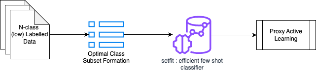
Semi-supervised classification with noise oversampling
Cascade this after the initial label subset formation — i.e., this classifier is only classifying between a given subset of classes.
Picture this: when you have low amounts of training data, you absolutely cannot create a hold-out set that is meaningful for evaluation. Should you do it at all? How do you know if your classifier is working well?
We approached this problem slightly differently — we defined the fundamental job of a semi-supervised classifier to be pre-emptive classification of a sample. This means that regardless of what a sample gets classified as it will be ‘verified’ and ‘corrected’ at a later stage: this classifier only needs to identify what needs to be verified.
As such, we created a design for how it would treat its data:
- n+1 classes, where the last class is noise
- noise: data from classes that are NOT in the current classifier’s purview. The noise class is oversampled to be 2x the average size of the data for the classifier’s labels
Oversampling on noise is a faux-safety measure, to ensure that adjacent data that belongs to another class is most likely predicted as noise instead of slipping through for verification.
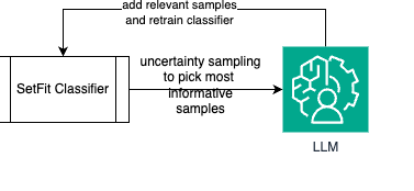
How do you check if this classifier is working well — in our experiments, we define this as the number of ‘uncertain’ samples in a classifier’s prediction. Using uncertainty sampling and information gain principles, we were effectively able to gauge if a classifier is ‘learning’ or not, which acts as a pointer towards classification performance. This classifier is consistently retrained unless there is an inflection point in the number of uncertain samples predicted, or there is only a delta of information being added iteratively by new samples.
Proxy active learning via an LLM agent
This is the heart of the approach — using an LLM as a proxy for a human validator. The human validator approach we are talking about is Active Labelling
Let’s get an intuitive understanding of Active Labelling:
- Use an ML model to learn on a sample input dataset, predict on a large set of datapoints
- For the predictions given on the datapoints, a subject-matter expert (SME) evaluates ‘validity’ of predictions
- Recursively, new ‘corrected’ samples are added as training data to the ML model
- The ML model consistently learns/retrains, and makes predictions until the SME is satisfied by the quality of predictions
For Active Labelling to work, there are expectations involved for an SME:
- when we expect a human expert to ‘validate’ an output sample, the expert understands what the task is
- a human expert will use judgement to evaluate ‘what else’ definitely belongs to a label L when deciding if a new sample should belong to L
Given these expectations and intuitions, we can ‘mimic’ these using an LLM:
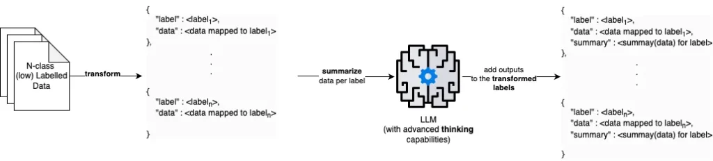
- give the LLM an ‘understanding’ of what each label means. This can be done by using a larger model to critically evaluate the relationship between {label: data mapped to label} for all labels. In our experiments, this was done using a 32B variant of DeepSeek that was self-hosted.
- Instead of predicting what is the correct label, leverage the LLM to identify if a prediction is ‘valid’ or ‘invalid’ only (i.e., LLM only has to answer a binary query).
- Reinforce the idea of what other valid samples for the label look like, i.e., for every pre-emptively predicted label for a sample, dynamically source c closest samples in its training (guaranteed valid) set when prompting for validation.
The result? A cost-effective framework that relies on a fast, cheap classifier to make pre-emptive classifications, and an LLM that verifies these using (meaning of the label + dynamically sourced training samples that are similar to the current classification):
import math

def calculate_uncertainty(clf, sample):
    predicted_probabilities = clf.predict_proba(sample.reshape(1, -1))[0]  # Reshape sample for predict_proba
    uncertainty = -sum(p * math.log(p, 2) for p in predicted_probabilities)
    return uncertainty


def select_informative_samples(clf, data, k):
    informative_samples = []
    uncertainties = [calculate_uncertainty(clf, sample) for sample in data]

    # Sort data by descending order of uncertainty
    sorted_data = sorted(zip(data, uncertainties), key=lambda x: x[1], reverse=True)

    # Get top k samples with highest uncertainty
    for sample, uncertainty in sorted_data[:k]:
        informative_samples.append(sample)

    return informative_samples


def proxy_label(clf, llm_judge, k, testing_data):
    #llm_judge - any LLM with a system prompt tuned for verifying if a sample belongs to a class. Expected output is a bool : True or False. True verifies the original classification, False refutes it
    predicted_classes = clf.predict(testing_data)

    # Select k most informative samples using uncertainty sampling
    informative_samples = select_informative_samples(clf, testing_data, k)

    # List to store correct samples
    voted_data = []

    # Evaluate informative samples with the LLM judge
    for sample in informative_samples:
        sample_index = testing_data.tolist().index(sample.tolist()) # changed from testing_data.index(sample) because of numpy array type issue
        predicted_class = predicted_classes[sample_index]

        # Check if LLM judge agrees with the prediction
        if llm_judge(sample, predicted_class):
            # If correct, add the sample to voted data
            voted_data.append(sample)

    # Return the list of correct samples with proxy labels
    return voted_data
By feeding the valid samples (voted_data) to our classifier under controlled parameters, we achieve the ‘recursive’ part of our algorithm:
By doing this, we were able to achieve close-to-human-expert validation numbers on controlled multi-class datasets. Experimentally, R.E.D. scales up to 1,000 classes while maintaining a competent degree of accuracy almost on par with human experts (90%+ agreement).
I believe this is a significant achievement in applied ML, and has real-world uses for production-grade expectations of cost, speed, scale, and adaptability. The technical report, publishing later this year, highlights relevant code samples as well as experimental setups used to achieve given results.
All images, unless otherwise noted, are by the author
Interested in more details? Reach out to me over Medium or email for a chat!