Stay Ahead, Stay ONMINE

Understanding Model Calibration: A Gentle Introduction & Visual Exploration

How Reliable Are Your Predictions? About To be considered reliable, a model must be calibrated so that its confidence in each decision closely reflects its true outcome. In this blog post we’ll take a look at the most commonly used definition for calibration and then dive into a frequently used evaluation measure for Model Calibration. […]

How Reliable Are Your Predictions?

About

To be considered reliable, a model must be calibrated so that its confidence in each decision closely reflects its true outcome. In this blog post we’ll take a look at the most commonly used definition for calibration and then dive into a frequently used evaluation measure for Model Calibration. We’ll then cover some of the drawbacks of this measure and how these surfaced the need for additional notions of calibration, which require their own new evaluation measures. This post is not intended to be an in-depth dissection of all works on calibration, nor does it focus on how to calibrate models. Instead, it is meant to provide a gentle introduction to the different notions and their evaluation measures as well as to re-highlight some issues with a measure that is still widely used to evaluate calibration.

Table of Contents

What is Calibration?

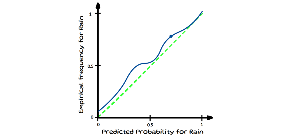
Calibration makes sure that a model’s estimated probabilities match real-world outcomes. For example, if a weather forecasting model predicts a 70% chance of rain on several days, then roughly 70% of those days should actually be rainy for the model to be considered well calibrated. This makes model predictions more reliable and trustworthy, which makes calibration relevant for many applications across various domains.

Reliability Diagram —  image by author

Now, what calibration means more precisely depends on the specific definition being considered. We will have a look at the most common notion in machine learning (ML) formalised by Guo and termed confidence calibration by Kull. But first, let’s define a bit of formal notation for this blog. 

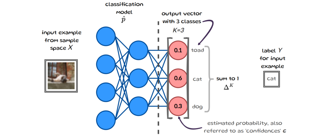
In this blog post we consider a classification task with K possible classes, with labels Y ∈ {1, …, K} and a classification model :𝕏 → Δᴷ, that takes inputs in 𝕏 (e.g. an image or text) and returns a probability vector as its output. Δᴷ refers to the K-simplex, which just means that the output vector must sum to 1 and that each estimated probability in the vector is between 0 & 1. These individual probabilities (or confidences) indicate how likely an input belongs to each of the K classes.

Notation — image by author — input example sourced from Uma

1.1 (Confidence) Calibration

A model is considered confidence-calibrated if, for all confidences c, the model is correct c proportion of the time:

where (X,Y) is a datapoint and p̂ : 𝕏 → Δᴷ returns a probability vector as its output

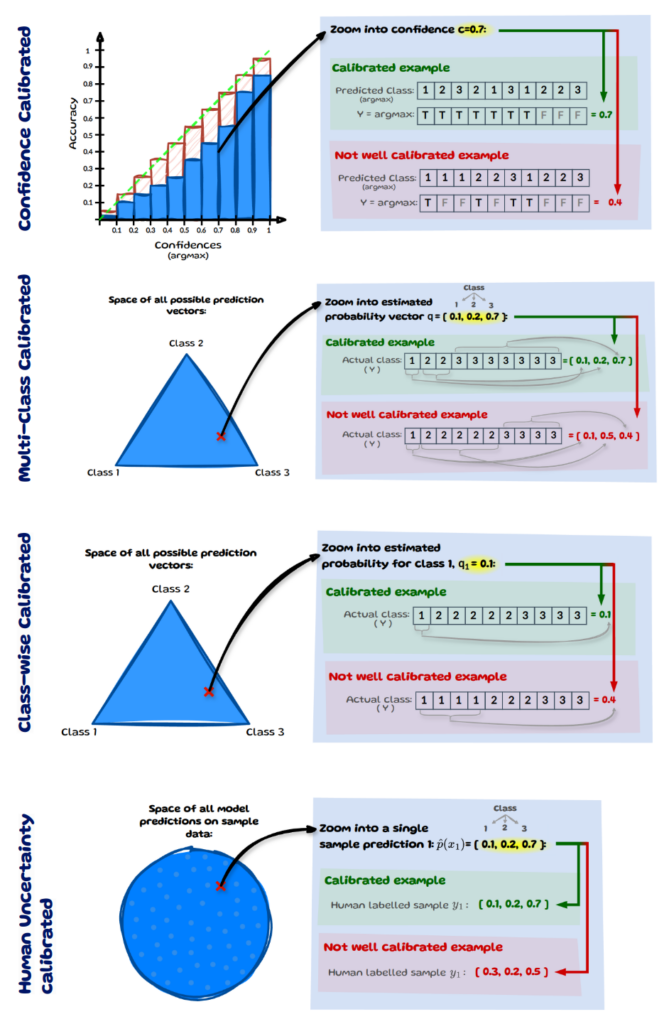
This definition of calibration, ensures that the model’s final predictions align with their observed accuracy at that confidence level. The left chart below visualises the perfectly calibrated outcome (green diagonal line) for all confidences using a binned reliability diagram. On the right hand side it shows two examples for a specific confidence level across 10 samples.

Confidence Calibration  —  image by author

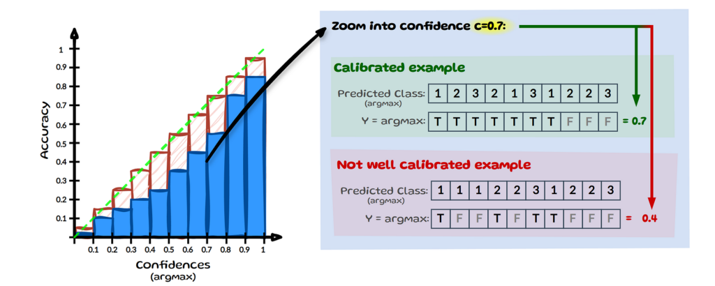
For simplification, we assume that we only have 3 classes as in image 2 (Notation) and we zoom into confidence c=0.7, see image above. Let’s assume we have 10 inputs here whose most confident prediction (max) equals 0.7. If the model correctly classifies 7 out of 10 predictions (true), it is considered calibrated at confidence level 0.7. For the model to be fully calibrated this has to hold across all confidence levels from 0 to 1. At the same level c=0.7, a model would be considered miscalibrated if it makes only 4 correct predictions.


2 Evaluating Calibration — Expected Calibration Error (ECE)

One widely used evaluation measure for confidence calibration is the Expected Calibration Error (ECE). ECE measures how well a model’s estimated probabilities match the observed probabilities by taking a weighted average over the absolute difference between average accuracy (acc) and average confidence (conf). The measure involves splitting all n datapoints into M equally spaced bins:

where B is used for representing “bins” and m for the bin number, while acc and conf are:

ŷᵢ is the model’s predicted class (arg max) for sample i and yᵢ is the true label for sample i. 1 is an indicator function, meaning when the predicted label ŷᵢ equals the true label yᵢ it evaluates to 1, otherwise 0. Let’s look at an example, which will clarify acc, conf and the whole binning approach in a visual step-by-step manner.

2.1 ECE — Visual Step by Step Example

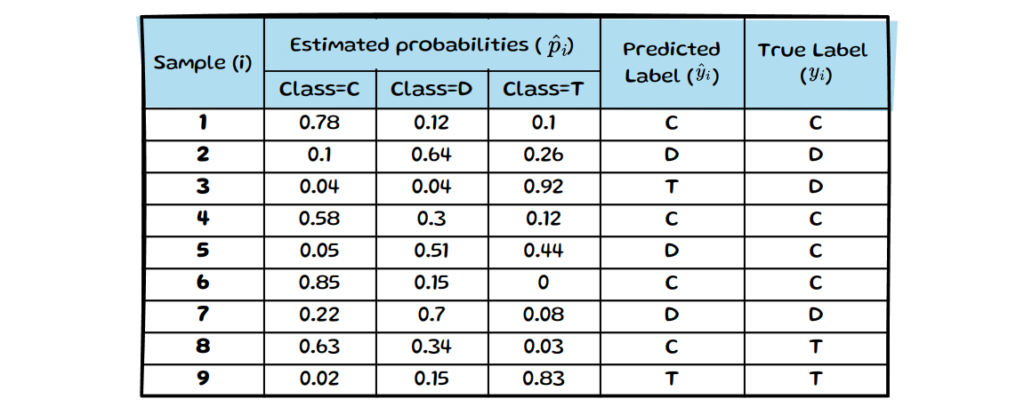
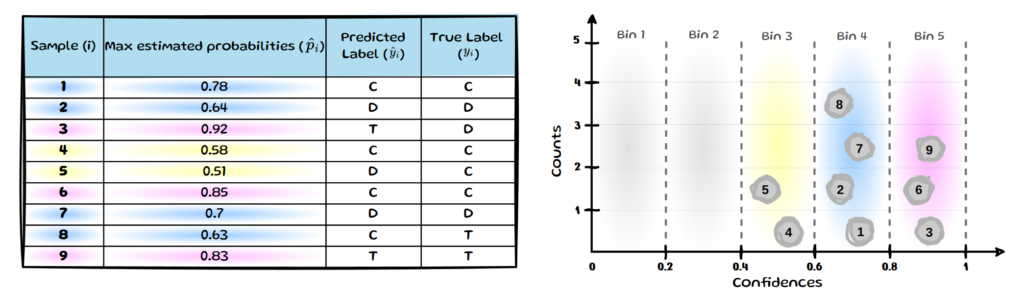
In the image below, we can see that we have 9 samples indexed by i with estimated probabilities p̂(xᵢ) (simplified as p̂ᵢ) for class cat (C), dog (D) or toad (T). The final column shows the true class yᵢ and the penultimate column contains the predicted class ŷᵢ.

Table 1 — ECE toy example — image by author

Only the maximum probabilities, which determine the predicted label are used in ECE. Therefore, we will only bin samples based on the maximum probability across classes (see left table in below image). To keep the example simple we split the data into 5 equally spaced bins M=5. If we now look at each sample’s maximum estimated probability, we can group it into one of the 5 bins (see right side of image below).

Table 2 & Binning Diagram — image by author

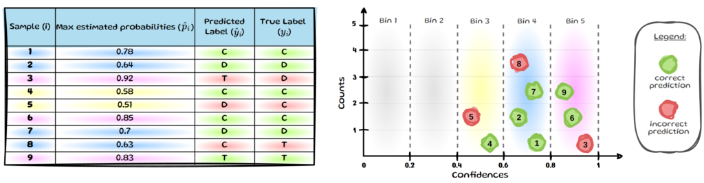
We still need to determine if the predicted class is correct or not to be able to determine the average accuracy per bin. If the model predicts the class correctly (i.e.  yᵢ = ŷᵢ), the prediction is highlighted in green; incorrect predictions are marked in red:

Table 3 & Binning Diagram — image by author

We now have visualised all the information needed for ECE and will briefly run through how to

calculate the values for bin 5 (B). The other bins then simply follow the same process, see below.

Table 4 & Example for bin 5  — image by author

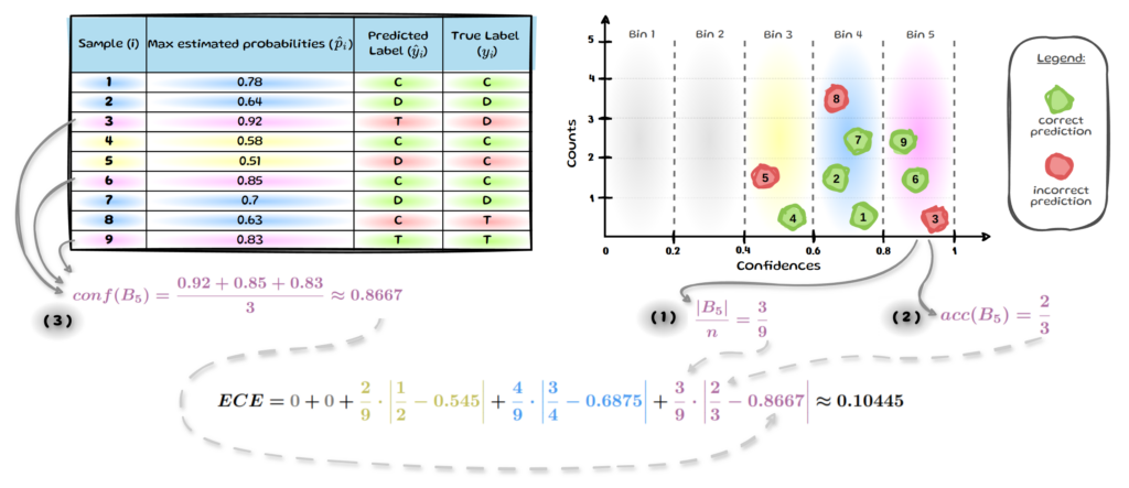
We can get the empirical probability of a sample falling into B, by assessing how many out of all 9 samples fall into B, see ( 1 ). We then get the average accuracy for B, see ( 2 ) and lastly the average estimated probability for B, see ( 3 ). Repeat this for all bins and in our small example of 9 samples we end up with an ECE of 0.10445. A perfectly calibrated model would have an ECE of 0.

For a more detailed, step-by-step explanation of the ECE, have a look at this blog post.

2.1.1  EXPECTED CALIBRATION ERROR DRAWBACKS

The images of binning above provide a visual guide of how ECE could result in very different values if we used more bins or perhaps binned the same number of items instead of using equal bin widths. Such and more drawbacks of ECE have been highlighted by several works early on. However, despite the known weaknesses ECE is still widely used to evaluate confidence calibration in ML. 

3 Most frequently mentioned Drawbacks of ECE

3.1 Pathologies — Low ECE ≠ high accuracy

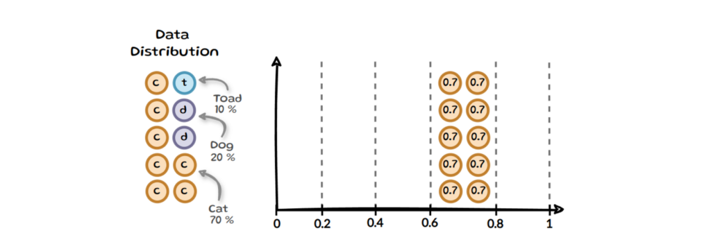
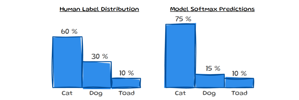
A model which minimises ECE, does not necessarily have a high accuracy. For instance, if a model always predicts the majority class with that class’s average prevalence as the probability, it will have an ECE of 0. This is visualised in the image above, where we have a dataset with 10 samples, 7 of those are cat, 2 dog and only one is a toad. Now if the model always predicts cat with on average 0.7 confidence it would have an ECE of 0. There are more of such pathologies. To not only rely on ECE, some researchers use additional measures such as the Brier score or LogLoss alongside ECE.

Sample Pathology —  image by author

3.2 Binning Approach

One of the most frequently mentioned issues with ECE is its sensitivity to the change in binning. This is sometimes referred to as the Bias-Variance trade-off: Fewer bins reduce variance but increase bias, while more bins lead to sparsely populated bins increasing variance. If we look back to our ECE example with 9 samples and change the bins from 5 to 10 here too, we end up with the following:

More Bins Example — image by author

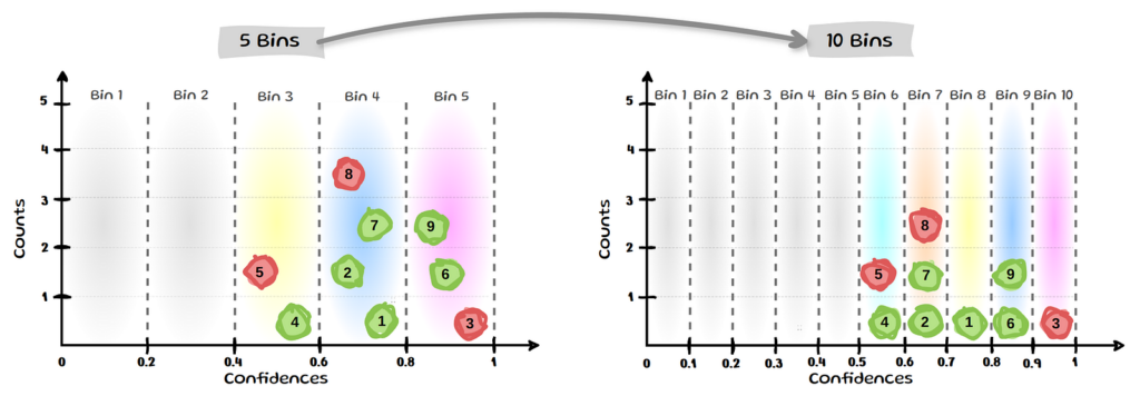
We can see that bin 8 and 9 each contain only a single sample and also that half the bins now contain no samples. The above is only a toy example, however since modern models tend to have higher confidence values samples often end up in the last few bins, which means they get all the weight in ECE, while the average error for the empty bins contributes 0 to ECE.

To mitigate these issues of fixed bin widths some authors have proposed a more adaptive binning approach:

Adaptive Bins Example — image by author

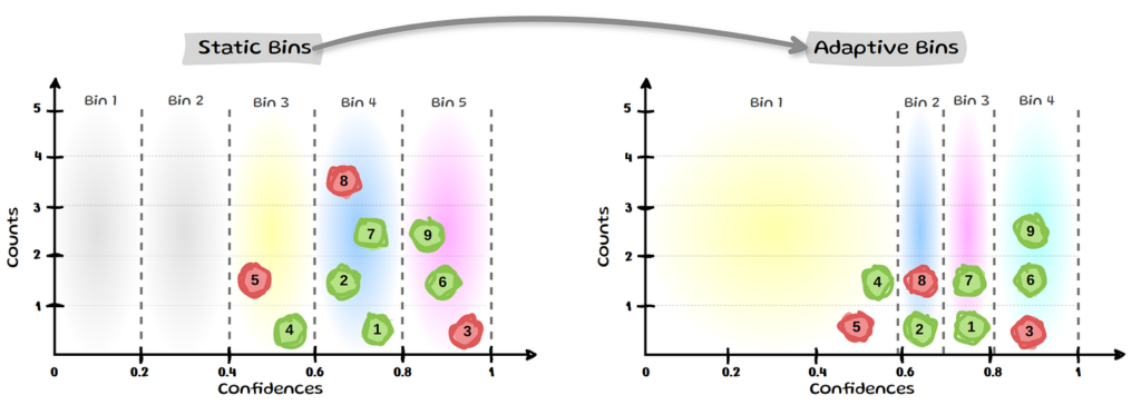
Binning-based evaluation with bins containing an equal number of samples are shown to have lower bias than a fixed binning approach such as ECE. This leads Roelofs to urge against using equal width binning and they suggest the use of an alternative: ECEsweep, which maximizes the number of equal-mass bins while ensuring the calibration function remains monotonic. The Adaptive Calibration Error (ACE) and Threshold Adaptive calibration Error (TACE) are two other variations of ECE that use flexible binning. However, some find it sensitive to the choice of bins and thresholds, leading to inconsistencies in ranking different models. Two other approaches aim to eliminate binning altogether: MacroCE does this by averaging over instance-level calibration errors of correct and wrong predictions and the KDE-based ECE does so by replacing the bins with non-parametric density estimators, specifically kernel density estimation (KDE).

3.3 Only maximum probabilities considered

Another frequently mentioned drawback of ECE is that it only considers the maximum estimated probabilities. The idea that more than just the maximum confidence should be calibrated, is best illustrated with a simple example:

Only Max. Probabilities — image by author — input example sourced from Schwirten

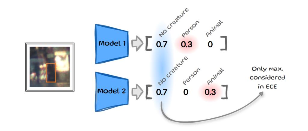
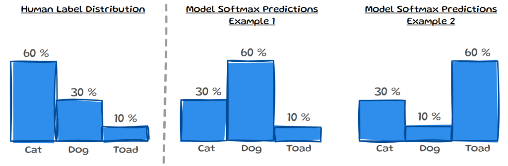
Let’s say we trained two different models and now both need to determine if the same input image contains a person, an animal or no creature. The two models output vectors with slightly different estimated probabilities, but both have the same maximum confidence for “no creature”. Since ECE only looks at these top values it would consider these two outputs to be the same. Yet, when we think of real-world applications we might want our self-driving car to act differently in one situation over the other. This restriction to the maximum confidence prompted various authors to reconsider the definition of calibration, which gives us two additional interpretations of confidence: multi-class and class-wise calibration.

3.3.1 MULTI-CLASS CALIBRATION

A model is considered multi-class calibrated if, for any prediction vector q=(q₁​,…,qₖ) ∈ Δᴷ​, the class proportions among all values of X for which a model outputs the same prediction p̂(X)=q match the values in the prediction vector q.

where (X,Y) is a datapoint and p̂ : 𝕏 → Δᴷ returns a probability vector as its output

What does this mean in simple terms? Instead of c we now calibrate against a vector q, with k classes. Let’s look at an example below:

Multi-Class Calibration — image by author

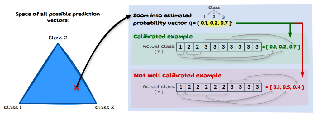
On the left we have the space of all possible prediction vectors. Let’s zoom into one such vector that our model predicted and say the model has 10 instances for which it predicted the vector q=[0.1,0.2,0.7]. Now in order for it to be multi-class calibrated, the distribution of the true (actual) class needs to match the prediction vector q. The image above shows a calibrated example with [0.1,0.2,0.7] and a not calibrated case with [0.1,0.5,0.4].

3.3.2 CLASS-WISE CALIBRATION

A model is considered class-wise calibrated if, for each class k, all inputs that share an estimated probability (X) align with the true frequency of class k when considered on its own:

where (X,Y) is a datapoint; q ∈ Δᴷ and p̂ : 𝕏 → Δᴷ returns a probability vector as its output

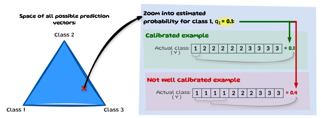
Class-wise calibration is a weaker definition than multi-class calibration as it considers each class probability in isolation rather than needing the full vector to align. The image below illustrates this by zooming into a probability estimate for class 1 specifically: q=0.1. Yet again, we assume we have 10 instances for which the model predicted a probability estimate of 0.1 for class 1. We then look at the true class frequency amongst all classes with q=0.1. If the empirical frequency matches q it is calibrated.

Class-Wise Calibration — image by author

To evaluate such different notions of calibration, some updates are made to ECE to calculate a class-wise error. One idea is to calculate the ECE for each class and then take the average. Others, introduce the use of the KS-test for class-wise calibration and also suggest using statistical hypothesis tests instead of ECE based approaches. And other researchers develop a hypothesis test framework (TCal) to detect whether a model is significantly mis-calibrated and build on this by developing confidence intervals for the L2 ECE.


All the approaches mentioned above share a key assumption: ground-truth labels are available. Within this gold-standard mindset a prediction is either true or false. However, annotators might unresolvably and justifiably disagree on the real label. Let’s look at a simple example below:

Gold-Standard Labelling | One-Hot-Vector —  image by author

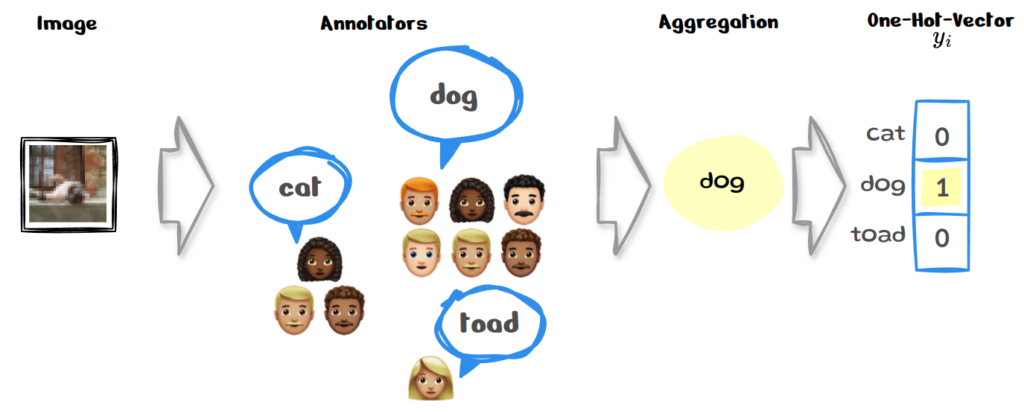
We have the same image as in our entry example and can see that the chosen label differs between annotators. A common approach to resolving such issues in the labelling process is to use some form of aggregation. Let’s say that in our example the majority vote is selected, so we end up evaluating how well our model is calibrated against such ‘ground truth’. One might think, the image is small and pixelated; of course humans will not be certain about their choice. However, rather than being an exception such disagreements are widespread. So, when there is a lot of human disagreement in a dataset it might not be a good idea to calibrate against an aggregated ‘gold’ label. Instead of gold labels more and more researchers are using soft or smooth labels which are more representative of the human uncertainty, see example below:

Collective Opinion Labelling | Soft-label — image by author

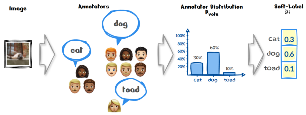
In the same example as above, instead of aggregating the annotator votes we could simply use their frequencies to create a distribution Pᵥₒₜₑ over the labels instead, which is then our new yᵢ. This shift towards training models on collective annotator views, rather than relying on a single source-of-truth motivates another definition of calibration: calibrating the model against human uncertainty.

3.3.3 HUMAN UNCERTAINTY CALIBRATION

A model is considered human-uncertainty calibrated if, for each specific sample x, the predicted probability for each class k matches the ‘actual’ probability Pᵥₒₜₑ of that class being correct.

where (X,Y) is a datapoint and p̂ : 𝕏 → Δᴷ returns a probability vector as its output.

This interpretation of calibration aligns the model’s prediction with human uncertainty, which means each prediction made by the model is individually reliable and matches human-level uncertainty for that instance. Let’s have a look at an example below:

Human Uncertainty Calibration — image by author

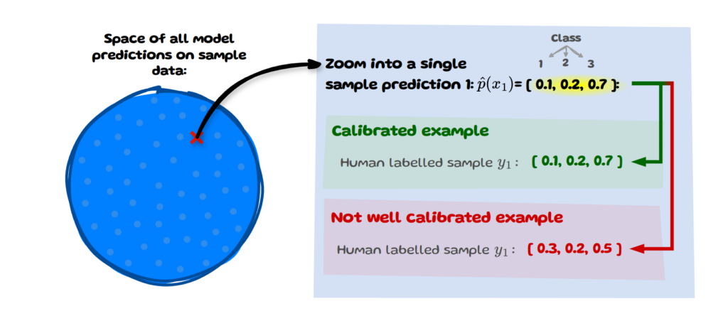
We have our sample data (left) and zoom into a single sample x with index i=1. The model’s predicted probability vector for this sample is [0.1,0.2,0.7]. If the human labelled distribution yᵢ matches this predicted vector then this sample is considered calibrated.

This definition of calibration is more granular and strict than the previous ones as it applies directly at the level of individual predictions rather than being averaged or assessed over a set of samples. It also relies heavily on having an accurate estimate of the human judgement distribution, which requires a large number of annotations per item. Datasets with such properties of annotations are gradually becoming more available.

To evaluate human uncertainty calibration the researchers introduce three new measures: the Human Entropy Calibration Error (EntCE), the Human Ranking Calibration Score (RankCS) and the Human Distribution Calibration Error (DistCE).

where H(.) signifies entropy.

EntCE aims to capture the agreement between the model’s uncertainty H(ᵢ) and the human uncertainty H(yᵢ) for a sample i. However, entropy is invariant to the permutations of the probability values; in other words it doesn’t change when you rearrange the probability values. This is visualised in the image below:

EntCE drawbacks — image by author

On the left, we can see the human label distribution yᵢ, on the right are two different model predictions for that same sample. All three distributions would have the same entropy, so comparing them would result in 0 EntCE. While this is not ideal for comparing distributions, entropy is still helpful in assessing the noise level of label distributions.

where argsort simply returns the indices that would sort an array.

So, RankCS checks if the sorted order of estimated probabilities p̂ᵢ matches the sorted order of yᵢ for each sample. If they match for a particular sample i one can count it as 1; if not, it can be counted as 0, which is then used to average over all samples N.¹

Since this approach uses ranking it doesn’t care about the actual size of the probability values. The two predictions below, while not the same in class probabilities would have the same ranking. This is helpful in assessing the overall ranking capability of models and looks beyond just the maximum confidence. At the same time though, it doesn’t fully capture human uncertainty calibration as it ignores the actual probability values.

RankCS drawbacks  — image by author

DistCE has been proposed as an additional evaluation for this notion of calibration. It simply uses the total variation distance (TVD) between the two distributions, which aims to reflect how much they diverge from one another. DistCE and EntCE capture instance level information. So to get a feeling for the full dataset one can simply take the average expected value over the absolute value of each measure: E[∣DistCE∣] and E[∣EntCE∣]. Perhaps future efforts will introduce further measures that combine the benefits of ranking and noise estimation for this notion of calibration.

4 Final thoughts

We have run through the most common definition of calibration, the shortcomings of ECE and how several new notions of calibration exist. We also touched on some of the newly proposed evaluation measures and their shortcomings. Despite several works arguing against the use of ECE for evaluating calibration, it remains widely used. The aim of this blog post is to draw attention to these works and their alternative approaches. Determining which notion of calibration best fits a specific context and how to evaluate it should avoid misleading results. Maybe, however, ECE is simply so easy, intuitive and just good enough for most applications that it is here to stay?

This was accepted at the ICLR conference Blog Post Track & is estimated to appear on the site ~ April

In the meantime, you can cite/reference the ArXiv preprint.

Footnotes

¹In the paper it is stated more generally: If the argsorts match, it means the ranking is aligned, contributing to the overall RankCS score.

Shape
Shape
Stay Ahead

Explore More Insights

Stay ahead with more perspectives on cutting-edge power, infrastructure, energy,  bitcoin and AI solutions. Explore these articles to uncover strategies and insights shaping the future of industries.

Shape

IBM proposes unified architecture for hybrid quantum-classical computing

Quantum computers and classical HPC are traditionally “disparate systems [that] operate in isolation,” IBM researchers explain in a new paper. This can be “cumbersome,” because users have to manually orchestrate workflows, coordinate scheduling, and transfer data between systems, thus hindering productivity and “severely” limiting algorithmic exploration. But a hybrid approach

Read More »

F5 brings new visibility and AI controls to Big-IP, NGINX

The demand came from a gap that general-purpose observability tools were not filling. Customers running tools like Datadog and New Relic told F5 they needed something different.  F5 Insight pulls from technology acquired through the Threat Stack and Fletch acquisitions and runs on F5’s AI data fabric. It includes an

Read More »

Tech layoffs surpass 45,000 in early 2026

Layoffs spread across tech sectors Beyond Amazon, Meta, and Block, several technology vendors and platform companies have also announced sizable layoffs this year. According to the RationalFX report: Semiconductor and electronics company ams OSRAM has announced 2,000 layoffs. Telecommunications vendor Ericsson has announced 1,900 job cuts. Semiconductor equipment manufacturer ASML

Read More »

Energy Department Announces $1.9B Investment in Critical Grid Infrastructure to Reduce Electricity Costs

WASHINGTON—The U.S. Department of Energy’s Office of Electricity (OE) today announced an approximately $1.9 billion funding opportunity to accelerate urgently needed upgrades to the nation’s power grid. These investments will meet rising electricity demand and resource adequacy needs, while lowering electricity costs for American households and businesses. Projects selected through the Speed to Power through Accelerated Reconductoring and other Key Advanced Transmission Technology Upgrades (SPARK) funding opportunity will deliver fast and durable upgrades to the grid with real results. In line with President Trump’s Executive Order, Unleashing American Energy, selected projects will demonstrate how reconductoring—replacing existing power lines with higher‑capacity conductors—paired with other Advanced Transmission Technologies (ATTs) can expand grid capacity, increase operational efficiency, lower prices for consumers, and improve overall system reliability and security of the nation’s electric grid. “For too long, important grid modernization and energy addition efforts were not prioritized by past leaders,” said U.S. Secretary of Energy Chris Wright. “Thanks to President Trump, we are doing the important work of modernizing our grid so electricity costs will be lowered for American families and businesses.” “The United States must increase grid capacity to meet demand, and ensure the grid provides reliable power—day-in and day-out,” said OE Assistant Secretary Katie Jereza. “Through this SPARK funding opportunity, we will stabilize and optimize grid operations to strengthen it for rapid growth.” The SPARK opportunity builds on the Grid Resilience and Innovation Partnerships (GRIP) Program, which provided up to $10.5 billion in competitive funding over five years to states, tribes, electric utilities, and other eligible recipients to strengthen grid resilience and innovation. The previous two GRIP funding rounds covered FY 2022-2023 and FY 2023-2024 funding. Today’s announcement continues the mission of the GRIP Program under the SPARK funding opportunity, focusing on the rapid deployment of reconductoring and other ATTs that expand transfer capability, strengthen reliability

Read More »

United States to Release 172 Million Barrels of Oil From the Strategic Petroleum Reserve

WASHINGTON—U.S. Secretary of Energy Chris Wright released the following statement regarding the International Energy Agency (IEA) and the U.S. Strategic Petroleum Reserve (SPR): “Earlier today, 32 member nations of the International Energy Agency unanimously agreed to President Trump’s request to lower energy prices with a coordinated release of 400 million barrels of oil and refined products from their respective reserves.  “As part of this effort, President Trump authorized the Department of Energy to release 172 million barrels from the Strategic Petroleum Reserve, beginning next week. This will take approximately 120 days to deliver based on planned discharge rates.  “President Trump promised to protect America’s energy security by managing the Strategic Petroleum Reserve responsibly and this action demonstrates his commitment to that promise. Unlike the previous administration, which left America’s oil reserves drained and damaged, the United States has arranged to more than replace these strategic reserves with approximately 200 million barrels within the next year—20% more barrels than will be drawn down—and at no cost to the taxpayer.  “For 47 years, Iran and its terrorist proxies have been intent on killing Americans. They have manipulated and threatened the energy security of America and its allies. Under President Trump, those days are coming to an end.  “Rest assured, America’s energy security is as strong as ever.”                                                                                         ###

Read More »

Occidental Petroleum, 1PointFive STRATOS DAC plant nears startup in Texas Permian basin

Occidental Petroleum Corp. and its subsidiary 1PointFive expect Phase 1 of the STRATOS direct air capture (DAC) plant in Texas’ Permian basin to come online in this year’s second quarter. In a post to LinkedIn, 1PointFive said Phase 1 “is in the final stage of startup” and that Phase 2, which incorporates learnings from research and development and Phase 1 construction activities, “will also begin commissioning in Q2, with operational ramp-up continuing through the rest of the year.” Once fully operational, STRATOS is designed to capture up to 500,000 tonnes/year (tpy) of CO2. As part of the US Environmental Protection Agency (EPA) Class VI permitting process and approval, it was reported that STRATOS is expected to include three wells to store about 722,000 tpy of CO2 in saline formations at a depth of about 4,400 ft. The company said a few activities before start-up remain, including ramping up remaining pellet reactors, completing calciner final commissioning in parallel, and beginning CO2 injection. Start-up milestones achieved include: Completed wet commissioning with water circulation. Received Class VI permits to sequester CO2. Ran CO2 compression system at design pressure. Added potassium hydroxide (KOH) to capture CO2 from the atmosphere. Building pellet inventory. Burners tested on calciner.  

Read More »

Brava Energia weighs Phase 3 at Atlanta to extend production plateau

Just 2 months after bringing its flagship Atlanta field onstream with the new FPSO Atlanta, Brazil’s independent operator Brava Energia SA is evaluating a potential third development phase that could add roughly 25 million bbl of reserves and help sustain peak production longer than originally planned. The Phase 3 project, still at an early technical and economic evaluation stage, focuses on the Atlanta Nordeste area; a separate, shallower reservoir discovered in 2006 by Shell’s 9-SHEL-19D-RJS well. According to André Fagundes, vice-president of research (Brazil) at Welligence Energy Analytics, Phase 2 has four wells still to be developed: two expected in 2027 and two in 2029. Phase 3 would involve drilling two additional wells in 2031, bringing total development to 12 producing wells. Until recently, full-field development was understood to comprise 10 wells, but Brava has since updated guidance to reflect a 12-well development concept. Atlanta field upside The primary objective is clear. “We believe its main objective is to extend the production plateau,” Fagundes said. Welligence estimates incremental recovery could reach 25 MMbbl, increasing the field’s overall recovery factor by roughly 1.5%. Lying outside Atlanta’s main Cretaceous reservoir, Atlanta Nordeste represents a genuine upside opportunity, Fagundes explained. The field benefits from strong natural aquifer support, and no water or gas injection is anticipated. Water-handling constraints that affected early production using the Petrojarl I—limited to 11,500 b/d of water treatment—are no longer a bottleneck. FPSO Atlanta can process up to 140,000 b/d of water. Reservoir performance to date has been solid, albeit with difficulties. Recurrent electric submersible pump (ESP) failures and processing limits on the previous FPSO complicated full validation of original reservoir models. With the new 50,000-b/d FPSO in operation since late 2024, reservoir deliverability has become the main constraint. Phase 3 wells would also use ESPs and require additional subsea

Read More »

California Resources eyes ‘measured’ capex ramp on way to 12% production growth thanks to Berry buy

@import url(‘https://fonts.googleapis.com/css2?family=Inter:[email protected]&display=swap’); a { color: var(–color-primary-main); } .ebm-page__main h1, .ebm-page__main h2, .ebm-page__main h3, .ebm-page__main h4, .ebm-page__main h5, .ebm-page__main h6 { font-family: Inter; } body { line-height: 150%; letter-spacing: 0.025em; font-family: Inter; } button, .ebm-button-wrapper { font-family: Inter; } .label-style { text-transform: uppercase; color: var(–color-grey); font-weight: 600; font-size: 0.75rem; } .caption-style { font-size: 0.75rem; opacity: .6; } #onetrust-pc-sdk [id*=btn-handler], #onetrust-pc-sdk [class*=btn-handler] { background-color: #c19a06 !important; border-color: #c19a06 !important; } #onetrust-policy a, #onetrust-pc-sdk a, #ot-pc-content a { color: #c19a06 !important; } #onetrust-consent-sdk #onetrust-pc-sdk .ot-active-menu { border-color: #c19a06 !important; } #onetrust-consent-sdk #onetrust-accept-btn-handler, #onetrust-banner-sdk #onetrust-reject-all-handler, #onetrust-consent-sdk #onetrust-pc-btn-handler.cookie-setting-link { background-color: #c19a06 !important; border-color: #c19a06 !important; } #onetrust-consent-sdk .onetrust-pc-btn-handler { color: #c19a06 !important; border-color: #c19a06 !important; } The leaders of California Resources Corp., Long Beach, plan to have the company’s total production average 152,000-157,000 boe/d in 2026, with each quarter expected to be in that range. That output would equate to an increase of more than 12% from the operator’s 137,000 boe/d during fourth-quarter 2025, due mostly to the mid-December acquisition of Berry Corp. Fourth-quarter results folded in 14 days of Berry production and included 109,000 b/d of oil, with the company’s assets in the San Joaquin and Los Angeles basins accounting for 99,000 b/d of that total. The company dilled 31 new wells during the quarter and 76 in all of 2025—all in the San Joaquin—but that number will grow significantly to about 260 this year as state officials have resumed issuing permits following the passage last fall of a bill focused on Kern County production. Speaking to analysts after CRC reported fourth-quarter net income of $12 million on $924 million in revenues, president and chief executive officer Francisco Leon and chief financial officer Clio Crespy said the goal is to manage 2026 output decline to roughly 0.5% per quarter while operating four rigs and

Read More »

Petro-Victory Energy spuds São João well in Brazil

@import url(‘https://fonts.googleapis.com/css2?family=Inter:[email protected]&display=swap’); a { color: var(–color-primary-main); } .ebm-page__main h1, .ebm-page__main h2, .ebm-page__main h3, .ebm-page__main h4, .ebm-page__main h5, .ebm-page__main h6 { font-family: Inter; } body { line-height: 150%; letter-spacing: 0.025em; font-family: Inter; } button, .ebm-button-wrapper { font-family: Inter; } .label-style { text-transform: uppercase; color: var(–color-grey); font-weight: 600; font-size: 0.75rem; } .caption-style { font-size: 0.75rem; opacity: .6; } #onetrust-pc-sdk [id*=btn-handler], #onetrust-pc-sdk [class*=btn-handler] { background-color: #c19a06 !important; border-color: #c19a06 !important; } #onetrust-policy a, #onetrust-pc-sdk a, #ot-pc-content a { color: #c19a06 !important; } #onetrust-consent-sdk #onetrust-pc-sdk .ot-active-menu { border-color: #c19a06 !important; } #onetrust-consent-sdk #onetrust-accept-btn-handler, #onetrust-banner-sdk #onetrust-reject-all-handler, #onetrust-consent-sdk #onetrust-pc-btn-handler.cookie-setting-link { background-color: #c19a06 !important; border-color: #c19a06 !important; } #onetrust-consent-sdk .onetrust-pc-btn-handler { color: #c19a06 !important; border-color: #c19a06 !important; } Petro-Victory Energy Corp. has spudded the SJ‑12 well at São João field in Barreirinhas basin, on the Brazilian equatorial margin, Maranhão.  Drilling and testing SJ‑12 is aimed at proving enough gas can be produced to sell locally. The well forms part of the single non‑associated gas well commitment under a memorandum of understanding signed in 2024 with Enava. São João contains 50.1 bcf (1.4 billion cu m) non‑associated gas resources. Petro‑Victory 100% owns and operates São João field.

Read More »

Cisco grows high-end optical support for AI clusters

Cisco has also upgraded its Network Conversion System (NCS) with a 1RU, 800GE line card offering 12.8T capacity, with 32 OSFP-based ports for 100GE, 400GE, and 800GE clients and 800ZR/ZR+ WDM trunks. The NCS 1014  doubles the density of previous-generation NCS versions and now includes MACsec encryption (IEEE 802.1AE) to secure point-to-point links with hardware-based encryption, data integrity, and authentication for Ethernet traffic, Ghioni stated. It supports enhanced capacity and performance with C&L-band support and NCS 1014 systems with the 2.4T WDM line card based on the Coherent Interconnect Module 8 and now supports 800 GE clients, which can be mapped directly to a wavelength or inverse multiplexed across two wavelengths to maximize reach, Ghioni wrote.  In the pluggable optic arena, Cisco is now offering a Quad Small Form Factor Pluggable Double Density (QSFP-DD) Pluggable Protection Switch Module that can monitor the optical link and switch traffic if it detects a fault in less than 50 milliseconds. The module occupies a quarter of the rack space compared to traditional protection devices—offering 90% rack space saving over available options, Ghioni wrote.  It is aimed at Metro and DCI network customers where sub-50 ms failure recovery is essential and data centers needing fiber protection without bulky hardware, Ghioni stated.  Cisco also added its Acacia developed Bright QSFP28 100ZR 0 dBm coherent optical pluggable in a standard QSFP28 form factor.  It is aimed at edge, access, enterprise, and campus network deployment. Cisco has been actively growing its optical portfolio  recently adding the Cisco Silicon One G300, which powers 102.4T N9000 and Cisco 8000 systems, as well as advanced 1.6T OSFP optics and 800G Linear Pluggable Optics. 

Read More »

Datalec targets rapid infrastructure deployment with new modular data centers

“We are engineering the data center with a new lens bringing pre-engineered system designs that are flexible and adaptable that enables a tailored solution for clients,” said John Lever, director of modular solutions at Datalec. The systems are flexible enough that these solutions cater for all types of data center, from standard server technology to AI and high-density compute. Datalec also provides “bolt-on” solutions, including a ‘digital wrapper’ including digital twinning and lifecycle and global support, Lever says. Another way Datalec says it differentiates from competing modular designs is a larger share of work is done offsite in a controlled manufacturing environment, which cuts onsite construction time, improves safety and limits disruption to live facilities, Lever says. The company competes with other modular data center vendors including Schneider Electric, Vertiv, Flex many others. DPI’s says its services are aimed at colocation providers, hyperscale and AI infrastructure teams, and large enterprises that need to add capacity quickly, safely and cost effectively across multiple regions.

Read More »

Study finds significant savings from direct current power for AI workloads

The result is a 50% to 80% reduction in copper usage, due to fewer conductors and less parallel cabling, and an 8% to 12% reduction in annual energy-related OpEx through lower conversion and distribution losses. By reducing conductor count, cabling, and redundant power components, 800VDC enables meaningful savings at both build-out and operational stages. AI-first facilities can see a $4 million to $8 million in CapEx savings per 10 MW build by reducing upstream AC. For a one-gigawatt data center, you’re saving a couple million pounds of copper wire, he said. Burke says an all-DC data center is best done with a whole new facility rather than retrofitting old facilities. “[DC] is going to be in a lot of greenfield data centers that are going to be built, and data centers that are going to go to higher compute power are also going to DC,” he said. He did recommend all-DC retrofits for existing data centers that are going to employ high power computing with GPUs. Enteligent’s unnamed and as yet unreleased product is a converter that takes 800 volts and partitions it to 50 volts for the computing servers. The company will provide a new power supply, power shelf that converts 800 volts DC to 50 volts DC much more efficiently than any current power supplies. Burke said the company is doing NDA level testing and pilot programs now with its product, but it will be making a formal announcement within the next few weeks. There are a number of players in the DC arena focusing on different parts of the power supply market including Vertiv, Rutherford, Siemens, Eaton and many more.

Read More »

Cisco blends Splunk analytics, security with core data center management

With the integration, data center teams can gather and act on events, alarms, health scores, and inventory through open APIs, Cisco stated. It also offers pre-built and customizable dashboards for inventory, health, fabric state, anomalies, and advisories as well as correlates telemetry across fabrics and technology tiers for actionable insights, according to Cisco. “This isn’t just another connector or API call. This is an embedded, architectural integration designed to transform how you monitor, troubleshoot, and secure your data center fabric. By bringing the power of Splunk directly into the Data Center Networking environment, we are enabling teams to solve complex problems faster, maintain strict data sovereignty, and dramatically reduce operational costs,” wrote Usha Andra is a senior product marketing leader and Anant Shah, senior product manager, both with Cisco Data Center Networking in a blog about the integration.  “Traditionally, network monitoring involves a trade-off. You either send massive amounts of raw logs to a centralized data lake, incurring high ingress and storage costs. Or you rely on sampled data that misses critical microbursts and anomalies,” Andra and Shah wrote.  “Native Splunk integration changes the paradigm by running Splunk capabilities directly within the Cisco Nexus Dashboard. This allows for the streaming of high-fidelity telemetry, including anomalies, advisories, and audit logs, directly to Splunk analytics.”

Read More »

Execution, Power, and Public Trust: Rich Miller on 2026’s Data Center Reality and Why He Built Data Center Richness

DCF founder Rich Miller has spent much of his career explaining how the data center industry works. Now, with his latest venture, Data Center Richness, he’s also examining how the industry learns. That thread provided the opening for the latest episode of The DCF Show Podcast, where Miller joined present Data Center Frontier Editor in Chief Matt Vincent and Senior Editor David Chernicoff for a wide-ranging discussion that ultimately landed on a simple conclusion: after two years of unprecedented AI-driven announcements, 2026 will be the year reality asserts itself. Projects will either get built, or they won’t. Power will either materialize, or it won’t. Communities will either accept data center expansion – or they’ll stop it. In other words, the industry is entering its execution phase. Why Data Center Richness Matters Now Miller launched Data Center Richness as both a podcast and a Substack publication, an effort to experiment with formats and better understand how professionals now consume industry information. Podcasts have become a primary way many practitioners follow the business, while YouTube’s discovery advantages increasingly make video versions essential. At the same time, Miller remains committed to written analysis, using Substack as a venue for deeper dives and format experimentation. One example is his weekly newsletter distilling key industry developments into just a handful of essential links rather than overwhelming readers with volume. The approach reflects a broader recognition: the pace of change has accelerated so much that clarity matters more than quantity. The topic of how people learn about data centers isn’t separate from the industry’s trajectory; it’s becoming part of it. Public perception, regulatory scrutiny, and investor expectations are now shaped by how stories are told as much as by how facilities are built. That context sets the stage for the conversation’s core theme. Execution Defines 2026 After

Read More »

Nomads at the Frontier: PTC 2026 Signals the Digital Infrastructure Industry’s Moment of Execution

Each January, the Pacific Telecommunications Council conference serves as a barometer for where digital infrastructure is headed next. And according to Nomad Futurist founders Nabeel Mahmood and Phillip Koblence, the message from PTC 2026 was unmistakable: The industry has moved beyond hype. The hard work has begun. In the latest episode of The DCF Show Podcast, part of our ongoing ‘Nomads at the Frontier’ series, Mahmood and Koblence joined Data Center Frontier to unpack the tone shift emerging across the AI and data center ecosystem. Attendance continues to grow year over year. Conversations remain energetic. But the character of those conversations has changed. As Mahmood put it: “The hype that the market started to see is actually resulting a bit more into actions now, and those conversations are resulting into some good progress.” The difference from prior years? Less speculation. More execution. From Data Center Cowboys to Real Deployments Koblence offered perhaps the sharpest contrast between PTC conversations in 2024 and those in 2026. Two years ago, many projects felt speculative. Today, developers are arriving with secured power, customers, and construction underway. “If 2024’s PTC was data center cowboys — sites that in someone’s mind could be a data center — this year was: show me the money, show me the power, give me accurate timelines.” In other words, the market is no longer rewarding hypothetical capacity. It is demanding delivered capacity. Operators now speak in terms of deployments already underway, not aspirational campuses still waiting on permits and power commitments. And behind nearly every conversation sits the same gating factor. Power. Power Has Become the Industry’s Defining Constraint Whether discussions centered on AI factories, investment capital, or campus expansion, Mahmood and Koblence noted that every conversation eventually returned to energy availability. “All of those questions are power,” Koblence said.

Read More »

Microsoft will invest $80B in AI data centers in fiscal 2025

And Microsoft isn’t the only one that is ramping up its investments into AI-enabled data centers. Rival cloud service providers are all investing in either upgrading or opening new data centers to capture a larger chunk of business from developers and users of large language models (LLMs).  In a report published in October 2024, Bloomberg Intelligence estimated that demand for generative AI would push Microsoft, AWS, Google, Oracle, Meta, and Apple would between them devote $200 billion to capex in 2025, up from $110 billion in 2023. Microsoft is one of the biggest spenders, followed closely by Google and AWS, Bloomberg Intelligence said. Its estimate of Microsoft’s capital spending on AI, at $62.4 billion for calendar 2025, is lower than Smith’s claim that the company will invest $80 billion in the fiscal year to June 30, 2025. Both figures, though, are way higher than Microsoft’s 2020 capital expenditure of “just” $17.6 billion. The majority of the increased spending is tied to cloud services and the expansion of AI infrastructure needed to provide compute capacity for OpenAI workloads. Separately, last October Amazon CEO Andy Jassy said his company planned total capex spend of $75 billion in 2024 and even more in 2025, with much of it going to AWS, its cloud computing division.

Read More »

John Deere unveils more autonomous farm machines to address skill labor shortage

Join our daily and weekly newsletters for the latest updates and exclusive content on industry-leading AI coverage. Learn More Self-driving tractors might be the path to self-driving cars. John Deere has revealed a new line of autonomous machines and tech across agriculture, construction and commercial landscaping. The Moline, Illinois-based John Deere has been in business for 187 years, yet it’s been a regular as a non-tech company showing off technology at the big tech trade show in Las Vegas and is back at CES 2025 with more autonomous tractors and other vehicles. This is not something we usually cover, but John Deere has a lot of data that is interesting in the big picture of tech. The message from the company is that there aren’t enough skilled farm laborers to do the work that its customers need. It’s been a challenge for most of the last two decades, said Jahmy Hindman, CTO at John Deere, in a briefing. Much of the tech will come this fall and after that. He noted that the average farmer in the U.S. is over 58 and works 12 to 18 hours a day to grow food for us. And he said the American Farm Bureau Federation estimates there are roughly 2.4 million farm jobs that need to be filled annually; and the agricultural work force continues to shrink. (This is my hint to the anti-immigration crowd). John Deere’s autonomous 9RX Tractor. Farmers can oversee it using an app. While each of these industries experiences their own set of challenges, a commonality across all is skilled labor availability. In construction, about 80% percent of contractors struggle to find skilled labor. And in commercial landscaping, 86% of landscaping business owners can’t find labor to fill open positions, he said. “They have to figure out how to do

Read More »

2025 playbook for enterprise AI success, from agents to evals

Join our daily and weekly newsletters for the latest updates and exclusive content on industry-leading AI coverage. Learn More 2025 is poised to be a pivotal year for enterprise AI. The past year has seen rapid innovation, and this year will see the same. This has made it more critical than ever to revisit your AI strategy to stay competitive and create value for your customers. From scaling AI agents to optimizing costs, here are the five critical areas enterprises should prioritize for their AI strategy this year. 1. Agents: the next generation of automation AI agents are no longer theoretical. In 2025, they’re indispensable tools for enterprises looking to streamline operations and enhance customer interactions. Unlike traditional software, agents powered by large language models (LLMs) can make nuanced decisions, navigate complex multi-step tasks, and integrate seamlessly with tools and APIs. At the start of 2024, agents were not ready for prime time, making frustrating mistakes like hallucinating URLs. They started getting better as frontier large language models themselves improved. “Let me put it this way,” said Sam Witteveen, cofounder of Red Dragon, a company that develops agents for companies, and that recently reviewed the 48 agents it built last year. “Interestingly, the ones that we built at the start of the year, a lot of those worked way better at the end of the year just because the models got better.” Witteveen shared this in the video podcast we filmed to discuss these five big trends in detail. Models are getting better and hallucinating less, and they’re also being trained to do agentic tasks. Another feature that the model providers are researching is a way to use the LLM as a judge, and as models get cheaper (something we’ll cover below), companies can use three or more models to

Read More »

OpenAI’s red teaming innovations define new essentials for security leaders in the AI era

Join our daily and weekly newsletters for the latest updates and exclusive content on industry-leading AI coverage. Learn More OpenAI has taken a more aggressive approach to red teaming than its AI competitors, demonstrating its security teams’ advanced capabilities in two areas: multi-step reinforcement and external red teaming. OpenAI recently released two papers that set a new competitive standard for improving the quality, reliability and safety of AI models in these two techniques and more. The first paper, “OpenAI’s Approach to External Red Teaming for AI Models and Systems,” reports that specialized teams outside the company have proven effective in uncovering vulnerabilities that might otherwise have made it into a released model because in-house testing techniques may have missed them. In the second paper, “Diverse and Effective Red Teaming with Auto-Generated Rewards and Multi-Step Reinforcement Learning,” OpenAI introduces an automated framework that relies on iterative reinforcement learning to generate a broad spectrum of novel, wide-ranging attacks. Going all-in on red teaming pays practical, competitive dividends It’s encouraging to see competitive intensity in red teaming growing among AI companies. When Anthropic released its AI red team guidelines in June of last year, it joined AI providers including Google, Microsoft, Nvidia, OpenAI, and even the U.S.’s National Institute of Standards and Technology (NIST), which all had released red teaming frameworks. Investing heavily in red teaming yields tangible benefits for security leaders in any organization. OpenAI’s paper on external red teaming provides a detailed analysis of how the company strives to create specialized external teams that include cybersecurity and subject matter experts. The goal is to see if knowledgeable external teams can defeat models’ security perimeters and find gaps in their security, biases and controls that prompt-based testing couldn’t find. What makes OpenAI’s recent papers noteworthy is how well they define using human-in-the-middle

Read More »