Stay Ahead, Stay ONMINE

No More Tableau Downtime: Metadata API for Proactive Data Health

In today’s world, the reliability of data solutions is everything. When we build dashboards and reports, one expects that the numbers reflected there are correct and up-to-date. Based on these numbers, insights are drawn and actions are taken. For any unforeseen reason, if the dashboards are broken or if the numbers are incorrect — then it becomes a fire-fight to fix everything. If the issues are not fixed in time, then it damages the trust placed on the data team and their solutions.  But why would dashboards be broken or have wrong numbers? If the dashboard was built correctly the first time, then 99% of the time the issue comes from the data that feeds the dashboards — from the data warehouse. Some possible scenarios are: Few ETL pipelines failed, so the new data is not yet in A table is replaced with another new one  Some columns in the table are dropped or renamed Schemas in data warehouse have changed And many more. There is still a chance that the issue is on the Tableau site, but in my experience, most of the times, it is always due to some changes in data warehouse. Even though we know the root cause, it’s not always straightforward to start working on a fix. There is no central place where you can check which Tableau data sources rely on specific tables. If you have the Tableau Data Management add-on, it could help, but from what I know, its hard to find dependencies of custom sql queries used in data sources. Nevertheless, the add-on is too expensive and most companies don’t have it. The real pain begins when you have to go through all the data sources manually to start fixing it. On top of it, you have a string of users on your head impatiently waiting for a quick-fix. The fix itself might not be difficult, it would just be a time-consuming one. What if we could anticipate these issues and identify impacted data sources before anyone notices a problem? Wouldn’t that just be great? Well, there is a way now with the Tableau Metadata API. The Metadata API uses GraphQL, a query language for APIs that returns only the data that you’re interested in. For more info on what’s possible with GraphQL, do check out GraphQL.org. In this blog post, I’ll show you how to connect to the Tableau Metadata API using Python’s Tableau Server Client (TSC) library to proactively identify data sources using specific tables, so that you can act fast before any issues arise. Once you know which Tableau data sources are affected by a specific table, you can make some updates yourself or alert the owners of those data sources about the upcoming changes so they can be prepared for it. Connecting to the Tableau Metadata API Lets connect to the Tableau Server using TSC. We need to import in all the libraries we would need for the exercise! ### Import all required libraries import tableauserverclient as t import pandas as pd import json import ast import re In order to connect to the Metadata API, you will have to first create a personal access token in your Tableau Account settings. Then update the & with the token you just created. Also update with your Tableau site. If the connection is established successfully, then “Connected” will be printed in the output window. ### Connect to Tableau server using personal access token tableau_auth = t.PersonalAccessTokenAuth(“”, “”, site_id=””) server = t.Server(“https://dub01.online.tableau.com/”, use_server_version=True) with server.auth.sign_in(tableau_auth): print(“Connected”) Lets now get a list of all data sources that are published on your site. There are many attributes you can fetch, but for the current use case, lets keep it simple and only get the id, name and owner contact information for every data source. This will be our master list to which we will add in all other information. ############### Get all the list of data sources on your Site all_datasources_query = “”” { publishedDatasources { name id owner { name email } } }””” with server.auth.sign_in(tableau_auth): result = server.metadata.query( all_datasources_query ) Since I want this blog to be focussed on how to proactively identify which data sources are affected by a specific table, I’ll not be going into the nuances of Metadata API. To better understand how the query works, you can refer to a very detailed Tableau’s own Metadata API documentation. One thing to note is that the Metadata API returns data in a JSON format. Depending on what you are querying, you’ll end up with multiple nested json lists and it can get very tricky to convert this into a pandas dataframe. For the above metadata query, you will end up with a result which would like below (this is mock data just to give you an idea of what the output looks like): { “data”: { “publishedDatasources”: [ { “name”: “Sales Performance DataSource”, “id”: “f3b1a2c4-1234-5678-9abc-1234567890ab”, “owner”: { “name”: “Alice Johnson”, “email”: “[email protected]” } }, { “name”: “Customer Orders DataSource”, “id”: “a4d2b3c5-2345-6789-abcd-2345678901bc”, “owner”: { “name”: “Bob Smith”, “email”: “[email protected]” } }, { “name”: “Product Returns and Profitability”, “id”: “c5e3d4f6-3456-789a-bcde-3456789012cd”, “owner”: { “name”: “Alice Johnson”, “email”: “[email protected]” } }, { “name”: “Customer Segmentation Analysis”, “id”: “d6f4e5a7-4567-89ab-cdef-4567890123de”, “owner”: { “name”: “Charlie Lee”, “email”: “[email protected]” } }, { “name”: “Regional Sales Trends (Custom SQL)”, “id”: “e7a5f6b8-5678-9abc-def0-5678901234ef”, “owner”: { “name”: “Bob Smith”, “email”: “[email protected]” } } ] } } We need to convert this JSON response into a dataframe so that its easy to work with. Notice that we need to extract the name and email of the owner from inside the owner object.  ### We need to convert the response into dataframe for easy data manipulation col_names = result[‘data’][‘publishedDatasources’][0].keys() master_df = pd.DataFrame(columns=col_names) for i in result[‘data’][‘publishedDatasources’]: tmp_dt = {k:v for k,v in i.items()} master_df = pd.concat([master_df, pd.DataFrame.from_dict(tmp_dt, orient=’index’).T]) # Extract the owner name and email from the owner object master_df[‘owner_name’] = master_df[‘owner’].apply(lambda x: x.get(‘name’) if isinstance(x, dict) else None) master_df[‘owner_email’] = master_df[‘owner’].apply(lambda x: x.get(’email’) if isinstance(x, dict) else None) master_df.reset_index(inplace=True) master_df.drop([‘index’,’owner’], axis=1, inplace=True) print(‘There are ‘, master_df.shape[0] , ‘ datasources in your site’) This is how the structure of master_df would look like: Sample output of code Once we have the main list ready, we can go ahead and start getting the names of the tables embedded in the data sources. If you are an avid Tableau user, you know that there are two ways to selecting tables in a Tableau data source — one is to directly choose the tables and establish a relation between them and the other is to use a custom sql query with one or more tables to achieve a new resultant table. Therefore, we need to address both the cases. Processing of Custom SQL query tables Below is the query to get the list of all custom SQLs used in the site along with their data sources. Notice that I have filtered the list to get only first 500 custom sql queries. In case there are more in your org, you will have to use an offset to get the next set of custom sql queries. There is also an option of using cursor method in Pagination when you want to fetch large list of results (refer here). For the sake of simplicity, I just use the offset method as I know, as there are less than 500 custom sql queries used on the site. # Get the data sources and the table names from all the custom sql queries used on your Site custom_table_query = “”” { customSQLTablesConnection(first: 500){ nodes { id name downstreamDatasources { name } query } } } “”” with server.auth.sign_in(tableau_auth): custom_table_query_result = server.metadata.query( custom_table_query ) Based on our mock data, this is how our output would look like: { “data”: { “customSQLTablesConnection”: { “nodes”: [ { “id”: “csql-1234”, “name”: “RegionalSales_CustomSQL”, “downstreamDatasources”: [ { “name”: “Regional Sales Trends (Custom SQL)” } ], “query”: “SELECT r.region_name, SUM(s.sales_amount) AS total_sales FROM ecommerce.sales_data.Sales s JOIN ecommerce.sales_data.Regions r ON s.region_id = r.region_id GROUP BY r.region_name” }, { “id”: “csql-5678”, “name”: “ProfitabilityAnalysis_CustomSQL”, “downstreamDatasources”: [ { “name”: “Product Returns and Profitability” } ], “query”: “SELECT p.product_category, SUM(s.profit) AS total_profit FROM ecommerce.sales_data.Sales s JOIN ecommerce.sales_data.Products p ON s.product_id = p.product_id GROUP BY p.product_category” }, { “id”: “csql-9101”, “name”: “CustomerSegmentation_CustomSQL”, “downstreamDatasources”: [ { “name”: “Customer Segmentation Analysis” } ], “query”: “SELECT c.customer_id, c.location, COUNT(o.order_id) AS total_orders FROM ecommerce.sales_data.Customers c JOIN ecommerce.sales_data.Orders o ON c.customer_id = o.customer_id GROUP BY c.customer_id, c.location” }, { “id”: “csql-3141”, “name”: “CustomerOrders_CustomSQL”, “downstreamDatasources”: [ { “name”: “Customer Orders DataSource” } ], “query”: “SELECT o.order_id, o.customer_id, o.order_date, o.sales_amount FROM ecommerce.sales_data.Orders o WHERE o.order_status = ‘Completed'” }, { “id”: “csql-3142”, “name”: “CustomerProfiles_CustomSQL”, “downstreamDatasources”: [ { “name”: “Customer Orders DataSource” } ], “query”: “SELECT c.customer_id, c.customer_name, c.segment, c.location FROM ecommerce.sales_data.Customers c WHERE c.active_flag = 1” }, { “id”: “csql-3143”, “name”: “CustomerReturns_CustomSQL”, “downstreamDatasources”: [ { “name”: “Customer Orders DataSource” } ], “query”: “SELECT r.return_id, r.order_id, r.return_reason FROM ecommerce.sales_data.Returns r” } ] } } } Just like before when we were creating the master list of data sources, here also we have nested json for the downstream data sources where we would need to extract only the “name” part of it. In the “query” column, the entire custom sql is dumped. If we use regex pattern, we can easily search for the names of the table used in the query. We know that the table names always come after FROM or a JOIN clause and they generally follow the format … The is optional and most of the times not used. There were some queries I found which used this format and I ended up only getting the database and schema names, and not the complete table name. Once we have extracted the names of the data sources and the names of the tables, we need to merge the rows per data source as there can be multiple custom sql queries used in a single data source. ### Convert the custom sql response into dataframe col_names = custom_table_query_result[‘data’][‘customSQLTablesConnection’][‘nodes’][0].keys() cs_df = pd.DataFrame(columns=col_names) for i in custom_table_query_result[‘data’][‘customSQLTablesConnection’][‘nodes’]: tmp_dt = {k:v for k,v in i.items()} cs_df = pd.concat([cs_df, pd.DataFrame.from_dict(tmp_dt, orient=’index’).T]) # Extract the data source name where the custom sql query was used cs_df[‘data_source’] = cs_df.downstreamDatasources.apply(lambda x: x[0][‘name’] if x and ‘name’ in x[0] else None) cs_df.reset_index(inplace=True) cs_df.drop([‘index’,’downstreamDatasources’], axis=1,inplace=True) ### We need to extract the table names from the sql query. We know the table name comes after FROM or JOIN clause # Note that the name of table can be of the format .. # Depending on the format of how table is called, you will have to modify the regex expression def extract_tables(sql): # Regex to match database.schema.table or schema.table, avoid alias pattern = r'(?:FROM|JOIN)s+((?:[w+]|w+).(?:[w+]|w+)(?:.(?:[w+]|w+))?)b’ matches = re.findall(pattern, sql, re.IGNORECASE) return list(set(matches)) # Unique table names cs_df[‘customSQLTables’] = cs_df[‘query’].apply(extract_tables) cs_df = cs_df[[‘data_source’,’customSQLTables’]] # We need to merge datasources as there can be multiple custom sqls used in the same data source cs_df = cs_df.groupby(‘data_source’, as_index=False).agg({ ‘customSQLTables’: lambda x: list(set(item for sublist in x for item in sublist)) # Flatten & make unique }) print(‘There are ‘, cs_df.shape[0], ‘datasources with custom sqls used in it’) After we perform all the above operations, this is how the structure of cs_df would look like: Sample output of code Processing of regular Tables in Data Sources Now we need to get the list of all the regular tables used in a datasource which are not a part of custom SQL. There are two ways to go about it. Either use the publishedDatasources object and check for upstreamTables or use DatabaseTable and check for upstreamDatasources. I’ll go by the first method because I want the results at a data source level (basically, I want some code ready to reuse when I want to check a specific data source in further detail). Here again, for the sake of simplicity, instead of going for pagination, I’m looping through each datasource to ensure I have everything. We get the upstreamTables inside of the field object so that has to be cleaned out. ############### Get the data sources with the regular table names used in your site ### Its best to extract the tables information for every data source and then merge the results. # Since we only get the table information nested under fields, in case there are hundreds of fields # used in a single data source, we will hit the response limits and will not be able to retrieve all the data. data_source_list = master_df.name.tolist() col_names = [‘name’, ‘id’, ‘extractLastUpdateTime’, ‘fields’] ds_df = pd.DataFrame(columns=col_names) with server.auth.sign_in(tableau_auth): for ds_name in data_source_list: query = “”” { publishedDatasources (filter: { name: “”””+ ds_name + “””” }) { name id extractLastUpdateTime fields { name upstreamTables { name } } } } “”” ds_name_result = server.metadata.query( query ) for i in ds_name_result[‘data’][‘publishedDatasources’]: tmp_dt = {k:v for k,v in i.items() if k != ‘fields’} tmp_dt[‘fields’] = json.dumps(i[‘fields’]) ds_df = pd.concat([ds_df, pd.DataFrame.from_dict(tmp_dt, orient=’index’).T]) ds_df.reset_index(inplace=True) This is how the structure of ds_df would look: Sample output of code We can need to flatten out the fields object and extract the field names as well as the table names. Since the table names will be repeating multiple times, we would have to deduplicate to keep only the unique ones. # Function to extract the values of fields and upstream tables in json lists def extract_values(json_list, key): values = [] for item in json_list: values.append(item[key]) return values ds_df[“fields”] = ds_df[“fields”].apply(ast.literal_eval) ds_df[‘field_names’] = ds_df.apply(lambda x: extract_values(x[‘fields’],’name’), axis=1) ds_df[‘upstreamTables’] = ds_df.apply(lambda x: extract_values(x[‘fields’],’upstreamTables’), axis=1) # Function to extract the unique table names def extract_upstreamTable_values(table_list): values = set()a for inner_list in table_list: for item in inner_list: if ‘name’ in item: values.add(item[‘name’]) return list(values) ds_df[‘upstreamTables’] = ds_df.apply(lambda x: extract_upstreamTable_values(x[‘upstreamTables’]), axis=1) ds_df.drop([“index”,”fields”], axis=1, inplace=True) Once we do the above operations, the final structure of ds_df would look something like this: Sample output of code We have all the pieces and now we just have to merge them together: ###### Join all the data together master_data = pd.merge(master_df, ds_df, how=”left”, on=[“name”,”id”]) master_data = pd.merge(master_data, cs_df, how=”left”, left_on=”name”, right_on=”data_source”) # Save the results to analyse further master_data.to_excel(“Tableau Data Sources with Tables.xlsx”, index=False) This is our final master_data: Sample Output of code Table-level Impact Analysis Let’s say there were some schema changes on the “Sales” table and you want to know which data sources will be impacted. Then you can simply write a small function which checks if a table is present in either of the two columns — upstreamTables or customSQLTables like below. def filter_rows_with_table(df, col1, col2, target_table): “”” Filters rows in df where target_table is part of any value in either col1 or col2 (supports partial match). Returns full rows (all columns retained). “”” return df[ df.apply( lambda row: (isinstance(row[col1], list) and any(target_table in item for item in row[col1])) or (isinstance(row[col2], list) and any(target_table in item for item in row[col2])), axis=1 ) ] # As an example filter_rows_with_table(master_data, ‘upstreamTables’, ‘customSQLTables’, ‘Sales’) Below is the output. You can see that 3 data sources will be impacted by this change. You can also alert the data source owners Alice and Bob in advance about this so they can start working on a fix before something breaks on the Tableau dashboards. Sample output of code You can check out the complete version of the code in my Github repository here. This is just one of the potential use-cases of the Tableau Metadata API. You can also extract the field names used in custom sql queries and add to the dataset to get a field-level impact analysis. One can also monitor the stale data sources with the extractLastUpdateTime to see if those have any issues or need to be archived if they are not used any more. We can also use the dashboards object to fetch information at a dashboard level. Final Thoughts If you have come this far, kudos. This is just one use case of automating Tableau data management. It’s time to reflect on your own work and think which of those other tasks you could automate to make your life easier. I hope this mini-project served as an enjoyable learning experience to understand the power of Tableau Metadata API. If you liked reading this, you might also like another one of my blog posts about Tableau, on some of the challenges I faced when dealing with big . Also do check out my previous blog where I explored building an interactive, database-powered app with Python, Streamlit, and SQLite. Before you go… Follow me so you don’t miss any new posts I write in future; you will find more of my articles on my . You can also connect with me on LinkedIn or Twitter!
In today’s world, the reliability of data solutions is everything. When we build dashboards and reports, one expects that the numbers reflected there are correct and up-to-date. Based on these numbers, insights are drawn and actions are taken. For any unforeseen reason, if the dashboards are broken or if the numbers are incorrect — then it becomes a fire-fight to fix everything. If the issues are not fixed in time, then it damages the trust placed on the data team and their solutions. 

But why would dashboards be broken or have wrong numbers? If the dashboard was built correctly the first time, then 99% of the time the issue comes from the data that feeds the dashboards — from the data warehouse. Some possible scenarios are:

  • Few ETL pipelines failed, so the new data is not yet in
  • A table is replaced with another new one 
  • Some columns in the table are dropped or renamed
  • Schemas in data warehouse have changed
  • And many more.

There is still a chance that the issue is on the Tableau site, but in my experience, most of the times, it is always due to some changes in data warehouse. Even though we know the root cause, it’s not always straightforward to start working on a fix. There is no central place where you can check which Tableau data sources rely on specific tables. If you have the Tableau Data Management add-on, it could help, but from what I know, its hard to find dependencies of custom sql queries used in data sources.

Nevertheless, the add-on is too expensive and most companies don’t have it. The real pain begins when you have to go through all the data sources manually to start fixing it. On top of it, you have a string of users on your head impatiently waiting for a quick-fix. The fix itself might not be difficult, it would just be a time-consuming one.

What if we could anticipate these issues and identify impacted data sources before anyone notices a problem? Wouldn’t that just be great? Well, there is a way now with the Tableau Metadata API. The Metadata API uses GraphQL, a query language for APIs that returns only the data that you’re interested in. For more info on what’s possible with GraphQL, do check out GraphQL.org.

In this blog post, I’ll show you how to connect to the Tableau Metadata API using Python’s Tableau Server Client (TSC) library to proactively identify data sources using specific tables, so that you can act fast before any issues arise. Once you know which Tableau data sources are affected by a specific table, you can make some updates yourself or alert the owners of those data sources about the upcoming changes so they can be prepared for it.

Connecting to the Tableau Metadata API

Lets connect to the Tableau Server using TSC. We need to import in all the libraries we would need for the exercise!

### Import all required libraries
import tableauserverclient as t
import pandas as pd
import json
import ast
import re

In order to connect to the Metadata API, you will have to first create a personal access token in your Tableau Account settings. Then update the & with the token you just created. Also update with your Tableau site. If the connection is established successfully, then “Connected” will be printed in the output window.

### Connect to Tableau server using personal access token
tableau_auth = t.PersonalAccessTokenAuth("", "", 
                                           site_id="")
server = t.Server("https://dub01.online.tableau.com/", use_server_version=True)

with server.auth.sign_in(tableau_auth):
        print("Connected")

Lets now get a list of all data sources that are published on your site. There are many attributes you can fetch, but for the current use case, lets keep it simple and only get the id, name and owner contact information for every data source. This will be our master list to which we will add in all other information.

############### Get all the list of data sources on your Site

all_datasources_query = """ {
  publishedDatasources {
    name
    id
    owner {
    name
    email
    }
  }
}"""
with server.auth.sign_in(tableau_auth):
    result = server.metadata.query(
        all_datasources_query
    )

Since I want this blog to be focussed on how to proactively identify which data sources are affected by a specific table, I’ll not be going into the nuances of Metadata API. To better understand how the query works, you can refer to a very detailed Tableau’s own Metadata API documentation.

One thing to note is that the Metadata API returns data in a JSON format. Depending on what you are querying, you’ll end up with multiple nested json lists and it can get very tricky to convert this into a pandas dataframe. For the above metadata query, you will end up with a result which would like below (this is mock data just to give you an idea of what the output looks like):

{
  "data": {
    "publishedDatasources": [
      {
        "name": "Sales Performance DataSource",
        "id": "f3b1a2c4-1234-5678-9abc-1234567890ab",
        "owner": {
          "name": "Alice Johnson",
          "email": "[email protected]"
        }
      },
      {
        "name": "Customer Orders DataSource",
        "id": "a4d2b3c5-2345-6789-abcd-2345678901bc",
        "owner": {
          "name": "Bob Smith",
          "email": "[email protected]"
        }
      },
      {
        "name": "Product Returns and Profitability",
        "id": "c5e3d4f6-3456-789a-bcde-3456789012cd",
        "owner": {
          "name": "Alice Johnson",
          "email": "[email protected]"
        }
      },
      {
        "name": "Customer Segmentation Analysis",
        "id": "d6f4e5a7-4567-89ab-cdef-4567890123de",
        "owner": {
          "name": "Charlie Lee",
          "email": "[email protected]"
        }
      },
      {
        "name": "Regional Sales Trends (Custom SQL)",
        "id": "e7a5f6b8-5678-9abc-def0-5678901234ef",
        "owner": {
          "name": "Bob Smith",
          "email": "[email protected]"
        }
      }
    ]
  }
}

We need to convert this JSON response into a dataframe so that its easy to work with. Notice that we need to extract the name and email of the owner from inside the owner object. 

### We need to convert the response into dataframe for easy data manipulation

col_names = result['data']['publishedDatasources'][0].keys()
master_df = pd.DataFrame(columns=col_names)

for i in result['data']['publishedDatasources']:
    tmp_dt = {k:v for k,v in i.items()}
    master_df = pd.concat([master_df, pd.DataFrame.from_dict(tmp_dt, orient='index').T])

# Extract the owner name and email from the owner object
master_df['owner_name'] = master_df['owner'].apply(lambda x: x.get('name') if isinstance(x, dict) else None)
master_df['owner_email'] = master_df['owner'].apply(lambda x: x.get('email') if isinstance(x, dict) else None)

master_df.reset_index(inplace=True)
master_df.drop(['index','owner'], axis=1, inplace=True)
print('There are ', master_df.shape[0] , ' datasources in your site')

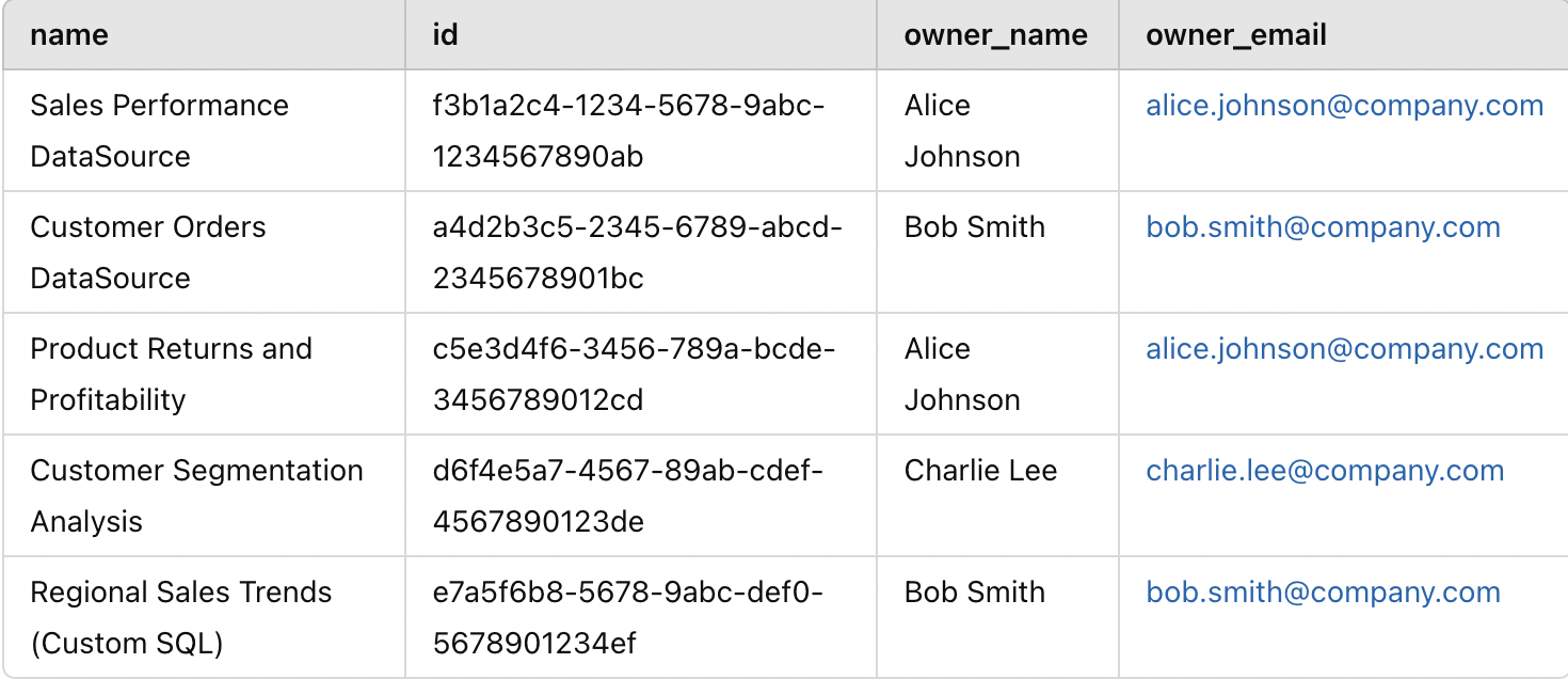
This is how the structure of master_df would look like:

Sample output of code

Once we have the main list ready, we can go ahead and start getting the names of the tables embedded in the data sources. If you are an avid Tableau user, you know that there are two ways to selecting tables in a Tableau data source — one is to directly choose the tables and establish a relation between them and the other is to use a custom sql query with one or more tables to achieve a new resultant table. Therefore, we need to address both the cases.

Processing of Custom SQL query tables

Below is the query to get the list of all custom SQLs used in the site along with their data sources. Notice that I have filtered the list to get only first 500 custom sql queries. In case there are more in your org, you will have to use an offset to get the next set of custom sql queries. There is also an option of using cursor method in Pagination when you want to fetch large list of results (refer here). For the sake of simplicity, I just use the offset method as I know, as there are less than 500 custom sql queries used on the site.

# Get the data sources and the table names from all the custom sql queries used on your Site

custom_table_query = """  {
  customSQLTablesConnection(first: 500){
    nodes {
        id
        name
        downstreamDatasources {
        name
        }
        query
    }
  }
}
"""

with server.auth.sign_in(tableau_auth):
    custom_table_query_result = server.metadata.query(
        custom_table_query
    )

Based on our mock data, this is how our output would look like:

{
  "data": {
    "customSQLTablesConnection": {
      "nodes": [
        {
          "id": "csql-1234",
          "name": "RegionalSales_CustomSQL",
          "downstreamDatasources": [
            {
              "name": "Regional Sales Trends (Custom SQL)"
            }
          ],
          "query": "SELECT r.region_name, SUM(s.sales_amount) AS total_sales FROM ecommerce.sales_data.Sales s JOIN ecommerce.sales_data.Regions r ON s.region_id = r.region_id GROUP BY r.region_name"
        },
        {
          "id": "csql-5678",
          "name": "ProfitabilityAnalysis_CustomSQL",
          "downstreamDatasources": [
            {
              "name": "Product Returns and Profitability"
            }
          ],
          "query": "SELECT p.product_category, SUM(s.profit) AS total_profit FROM ecommerce.sales_data.Sales s JOIN ecommerce.sales_data.Products p ON s.product_id = p.product_id GROUP BY p.product_category"
        },
        {
          "id": "csql-9101",
          "name": "CustomerSegmentation_CustomSQL",
          "downstreamDatasources": [
            {
              "name": "Customer Segmentation Analysis"
            }
          ],
          "query": "SELECT c.customer_id, c.location, COUNT(o.order_id) AS total_orders FROM ecommerce.sales_data.Customers c JOIN ecommerce.sales_data.Orders o ON c.customer_id = o.customer_id GROUP BY c.customer_id, c.location"
        },
        {
          "id": "csql-3141",
          "name": "CustomerOrders_CustomSQL",
          "downstreamDatasources": [
            {
              "name": "Customer Orders DataSource"
            }
          ],
          "query": "SELECT o.order_id, o.customer_id, o.order_date, o.sales_amount FROM ecommerce.sales_data.Orders o WHERE o.order_status = 'Completed'"
        },
        {
          "id": "csql-3142",
          "name": "CustomerProfiles_CustomSQL",
          "downstreamDatasources": [
            {
              "name": "Customer Orders DataSource"
            }
          ],
          "query": "SELECT c.customer_id, c.customer_name, c.segment, c.location FROM ecommerce.sales_data.Customers c WHERE c.active_flag = 1"
        },
        {
          "id": "csql-3143",
          "name": "CustomerReturns_CustomSQL",
          "downstreamDatasources": [
            {
              "name": "Customer Orders DataSource"
            }
          ],
          "query": "SELECT r.return_id, r.order_id, r.return_reason FROM ecommerce.sales_data.Returns r"
        }
      ]
    }
  }
}

Just like before when we were creating the master list of data sources, here also we have nested json for the downstream data sources where we would need to extract only the “name” part of it. In the “query” column, the entire custom sql is dumped. If we use regex pattern, we can easily search for the names of the table used in the query.

We know that the table names always come after FROM or a JOIN clause and they generally follow the format ..

. The is optional and most of the times not used. There were some queries I found which used this format and I ended up only getting the database and schema names, and not the complete table name. Once we have extracted the names of the data sources and the names of the tables, we need to merge the rows per data source as there can be multiple custom sql queries used in a single data source.

### Convert the custom sql response into dataframe
col_names = custom_table_query_result['data']['customSQLTablesConnection']['nodes'][0].keys()
cs_df = pd.DataFrame(columns=col_names)

for i in custom_table_query_result['data']['customSQLTablesConnection']['nodes']:
    tmp_dt = {k:v for k,v in i.items()}

    cs_df = pd.concat([cs_df, pd.DataFrame.from_dict(tmp_dt, orient='index').T])

# Extract the data source name where the custom sql query was used
cs_df['data_source'] = cs_df.downstreamDatasources.apply(lambda x: x[0]['name'] if x and 'name' in x[0] else None)
cs_df.reset_index(inplace=True)
cs_df.drop(['index','downstreamDatasources'], axis=1,inplace=True)

### We need to extract the table names from the sql query. We know the table name comes after FROM or JOIN clause
# Note that the name of table can be of the format ..
# Depending on the format of how table is called, you will have to modify the regex expression

def extract_tables(sql):
    # Regex to match database.schema.table or schema.table, avoid alias
    pattern = r'(?:FROM|JOIN)s+((?:[w+]|w+).(?:[w+]|w+)(?:.(?:[w+]|w+))?)b'
    matches = re.findall(pattern, sql, re.IGNORECASE)
    return list(set(matches))  # Unique table names

cs_df['customSQLTables'] = cs_df['query'].apply(extract_tables)
cs_df = cs_df[['data_source','customSQLTables']]

# We need to merge datasources as there can be multiple custom sqls used in the same data source
cs_df = cs_df.groupby('data_source', as_index=False).agg({
    'customSQLTables': lambda x: list(set(item for sublist in x for item in sublist))  # Flatten & make unique
})

print('There are ', cs_df.shape[0], 'datasources with custom sqls used in it')

After we perform all the above operations, this is how the structure of cs_df would look like:
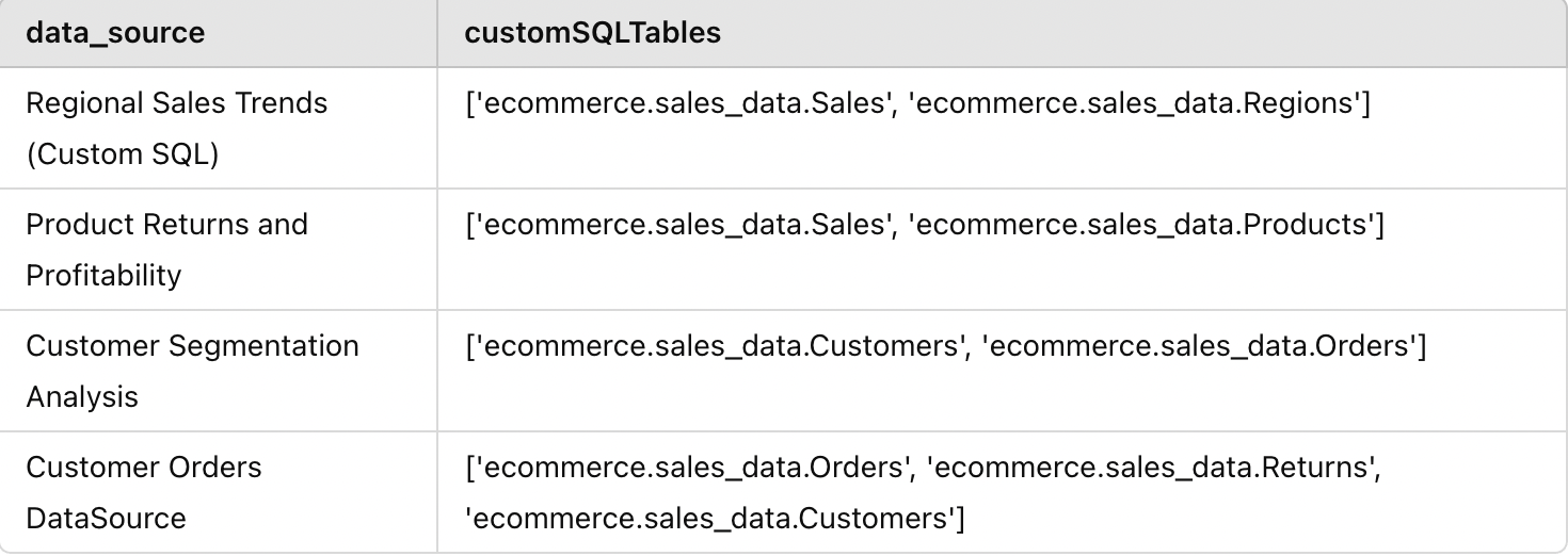
Sample output of code

Processing of regular Tables in Data Sources

Now we need to get the list of all the regular tables used in a datasource which are not a part of custom SQL. There are two ways to go about it. Either use the publishedDatasources object and check for upstreamTables or use DatabaseTable and check for upstreamDatasources. I’ll go by the first method because I want the results at a data source level (basically, I want some code ready to reuse when I want to check a specific data source in further detail). Here again, for the sake of simplicity, instead of going for pagination, I’m looping through each datasource to ensure I have everything. We get the upstreamTables inside of the field object so that has to be cleaned out.

############### Get the data sources with the regular table names used in your site

### Its best to extract the tables information for every data source and then merge the results.
# Since we only get the table information nested under fields, in case there are hundreds of fields 
# used in a single data source, we will hit the response limits and will not be able to retrieve all the data.

data_source_list = master_df.name.tolist()

col_names = ['name', 'id', 'extractLastUpdateTime', 'fields']
ds_df = pd.DataFrame(columns=col_names)

with server.auth.sign_in(tableau_auth):
    for ds_name in data_source_list:
        query = """ {
            publishedDatasources (filter: { name: """"+ ds_name + """" }) {
            name
            id
            extractLastUpdateTime
            fields {
                name
                upstreamTables {
                    name
                }
            }
            }
        } """
        ds_name_result = server.metadata.query(
        query
        )
        for i in ds_name_result['data']['publishedDatasources']:
            tmp_dt = {k:v for k,v in i.items() if k != 'fields'}
            tmp_dt['fields'] = json.dumps(i['fields'])
        ds_df = pd.concat([ds_df, pd.DataFrame.from_dict(tmp_dt, orient='index').T])

ds_df.reset_index(inplace=True)

This is how the structure of ds_df would look:
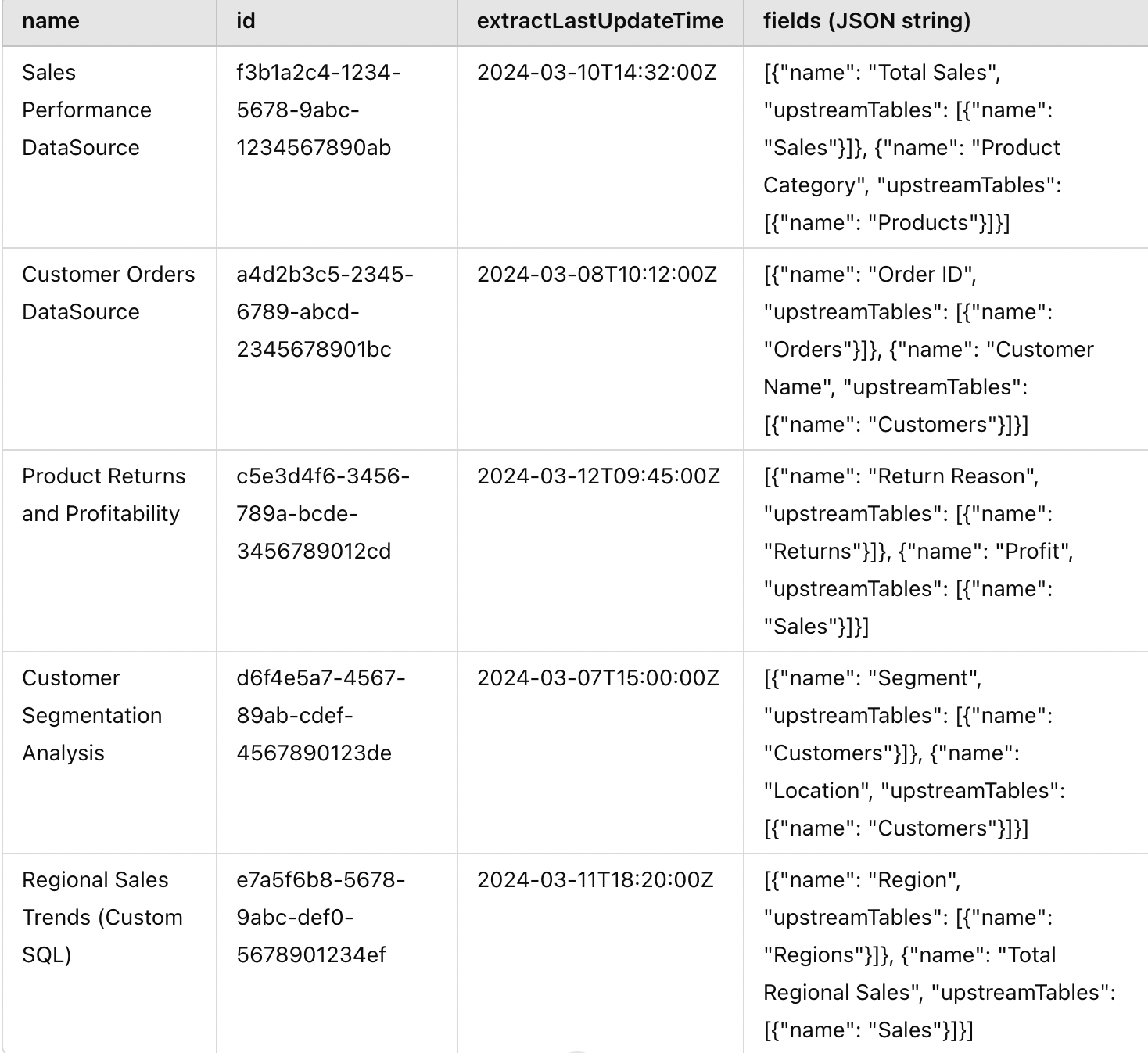
Sample output of code

We can need to flatten out the fields object and extract the field names as well as the table names. Since the table names will be repeating multiple times, we would have to deduplicate to keep only the unique ones.

# Function to extract the values of fields and upstream tables in json lists
def extract_values(json_list, key):
    values = []
    for item in json_list:
        values.append(item[key])
    return values

ds_df["fields"] = ds_df["fields"].apply(ast.literal_eval)
ds_df['field_names'] = ds_df.apply(lambda x: extract_values(x['fields'],'name'), axis=1)
ds_df['upstreamTables'] = ds_df.apply(lambda x: extract_values(x['fields'],'upstreamTables'), axis=1)

# Function to extract the unique table names 
def extract_upstreamTable_values(table_list):
    values = set()a
    for inner_list in table_list:
        for item in inner_list:
            if 'name' in item:
                values.add(item['name'])
    return list(values)

ds_df['upstreamTables'] = ds_df.apply(lambda x: extract_upstreamTable_values(x['upstreamTables']), axis=1)
ds_df.drop(["index","fields"], axis=1, inplace=True)

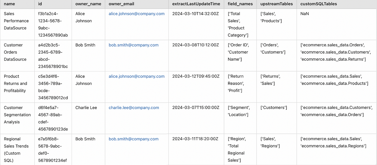
Once we do the above operations, the final structure of ds_df would look something like this:
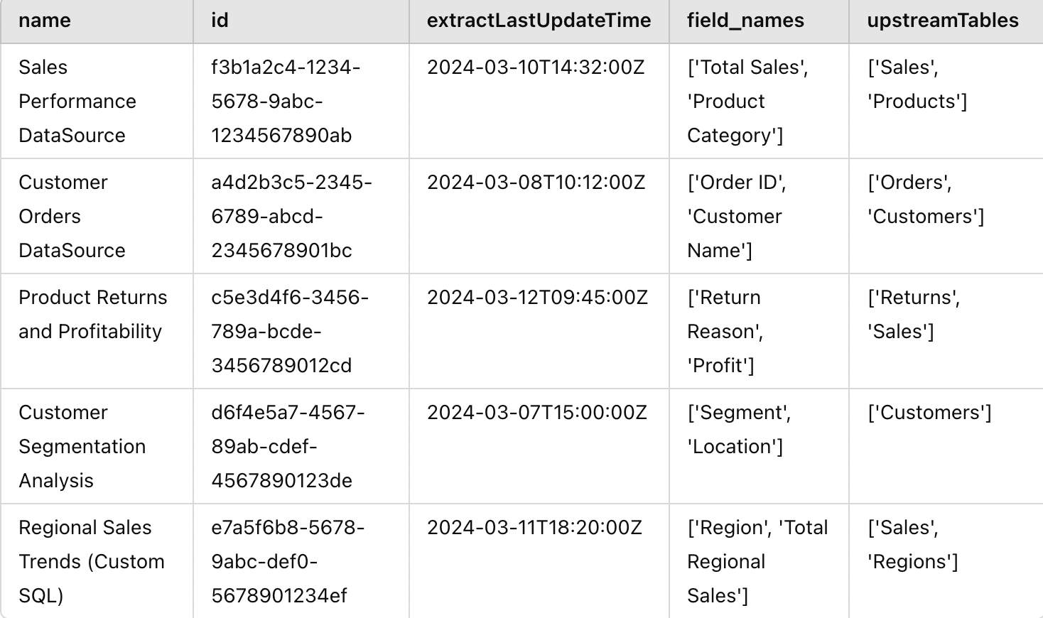
Sample output of code

We have all the pieces and now we just have to merge them together:

###### Join all the data together
master_data = pd.merge(master_df, ds_df, how="left", on=["name","id"])
master_data = pd.merge(master_data, cs_df, how="left", left_on="name", right_on="data_source")

# Save the results to analyse further
master_data.to_excel("Tableau Data Sources with Tables.xlsx", index=False)

This is our final master_data:

Sample Output of code

Table-level Impact Analysis

Let’s say there were some schema changes on the “Sales” table and you want to know which data sources will be impacted. Then you can simply write a small function which checks if a table is present in either of the two columns — upstreamTables or customSQLTables like below.

def filter_rows_with_table(df, col1, col2, target_table):
    """
    Filters rows in df where target_table is part of any value in either col1 or col2 (supports partial match).
    Returns full rows (all columns retained).
    """
    return df[
        df.apply(
            lambda row: 
                (isinstance(row[col1], list) and any(target_table in item for item in row[col1])) or
                (isinstance(row[col2], list) and any(target_table in item for item in row[col2])),
            axis=1
        )
    ]
# As an example 
filter_rows_with_table(master_data, 'upstreamTables', 'customSQLTables', 'Sales')

Below is the output. You can see that 3 data sources will be impacted by this change. You can also alert the data source owners Alice and Bob in advance about this so they can start working on a fix before something breaks on the Tableau dashboards.

Sample output of code

You can check out the complete version of the code in my Github repository here.

This is just one of the potential use-cases of the Tableau Metadata API. You can also extract the field names used in custom sql queries and add to the dataset to get a field-level impact analysis. One can also monitor the stale data sources with the extractLastUpdateTime to see if those have any issues or need to be archived if they are not used any more. We can also use the dashboards object to fetch information at a dashboard level.

Final Thoughts

If you have come this far, kudos. This is just one use case of automating Tableau data management. It’s time to reflect on your own work and think which of those other tasks you could automate to make your life easier. I hope this mini-project served as an enjoyable learning experience to understand the power of Tableau Metadata API. If you liked reading this, you might also like another one of my blog posts about Tableau, on some of the challenges I faced when dealing with big .

Also do check out my previous blog where I explored building an interactive, database-powered app with Python, Streamlit, and SQLite.


Before you go…

Follow me so you don’t miss any new posts I write in future; you will find more of my articles on my . You can also connect with me on LinkedIn or Twitter!

Shape
Shape
Stay Ahead

Explore More Insights

Stay ahead with more perspectives on cutting-edge power, infrastructure, energy,  bitcoin and AI solutions. Explore these articles to uncover strategies and insights shaping the future of industries.

Shape

IP Fabric 7.9 boosts visibility across hybrid environments

Multicloud and hybrid network viability has also been extended to include IPv6 path analysis, helping teams reason about connectivity in dual-stack and hybrid environments. This capability addresses a practical challenge for enterprises deploying IPv6 alongside existing IPv4 infrastructure. Network teams can now validate that applications can reach IPv6 endpoints and

Read More »

Kolibri Reports Increased Flows at New Oklahoma Wells

Kolibri Global Energy Inc has reported improved flow rates at the Barnes and Velin wells in Oklahoma’s Tishomingo field. The 1.5-mile lateral Barnes 6-31-2H well posted a 30-day average of 529 barrels of oil equivalent per day (boepd). The one-mile lateral Barnes 6-4H well averaged 452 boepd in 30 days, Thousand Oaks, California-based Kolibri said in a press release. The company said it owns 100 percent of the wells. “The Barnes wells continue to produce high percentages of oil (~83 percent), much like the Lovina wells the company drilled earlier this year” in the same field, Kolibri said. “On a comparable lateral length basis, these wells are producing at a boepd rate that is 22 percent higher than the Lovina wells were producing at the same time in their production life”, it added. Meanwhile the one-mile lateral wells Velin 12-9H and Velin 12-10H yielded 30-day averages of 257 boepd and 176 boepd respectively. Kolibri said it holds stakes of 97 percent in the wells. “The Velin wells are still improving and continue to act differently than the typical wells in the field”, Kolibri said. “There are some differences between these wells and the company’s offsetting wells. “One is that the Velin wells were shut in longer than our normal time after fracture stimulations were complete. This was due to the close proximity of all four wellbores, and as a result, the wells needed to stay shut-in while the Barnes wells were being fracture-stimulated. While that is standard industry practice, it may be a contributing factor to the lower early production rates and the slower cleanup. “Additionally, while the formation analysis of these wells is comparable to that of the offsetting wells, there is the presence of increased natural healed fractures and small-scale faulting, which appears unique to this location, potentially

Read More »

Veteran Gas Executive Leaving Mercuria

Steve Hill, who was hired by Mercuria Energy Group in 2024 to build out its liquefied natural gas business, is leaving the trading house. Hill was part of the company’s efforts to expand into the fast-growing global LNG market. Before joining, he was responsible for the vast LNG, gas and power marketing and trading business at energy giant Shell Plc. He was one of a trio of heavyweight hires Mercuria made after reaping bumper profits, setting off a renewed push into trading physical commodities, along with Kostas Bintas in metals and Nick O’Kane in gas and power. Known as one of the world’s biggest traders of oil and gas, the firm has been a relative latecomer behind other trading house rivals in building out a large-scale physical trading business for LNG. During Hill’s relatively brief tenure, Mercuria signed deals to offtake LNG from Oman, as well as supply Turkey and China. He also hired several of his former colleagues from Shell, though one — Singapore-based Dong Yuan — recently left the company. A spokesperson for Mercuria confirmed Hill is leaving the company. Hill didn’t immediately respond to a request for comment. WHAT DO YOU THINK? Generated by readers, the comments included herein do not reflect the views and opinions of Rigzone. All comments are subject to editorial review. Off-topic, inappropriate or insulting comments will be removed.

Read More »

Crude Settles Higher After Volatile Week

Oil edged higher at the end of a volatile week, as traders weighed tensions in Iran and positive sentiment in wider markets. West Texas Intermediate settled near $60 a barrel after plunging 4.6% on Thursday, the most since June. President Donald Trump said in a social media post that he “greatly” respects Iran’s decision to cancel scheduled hangings of protesters. His rhetoric over recent days has reduced expectations of an immediate US response to violent protests in the Islamic Republic, which could have led to disruptions to the country’s roughly 3.3 million barrel-per-day oil production, as well as shipping. Nevertheless, Washington is boosting its military presence in the Middle East. At least one aircraft carrier is moving into the region and other military assets are expected to be shifted there in the coming days and weeks, Fox News reported, citing military sources. Traders have in the past covered bearish wagers ahead of the weekend in periods of heightened geopolitical risks. “While the risk of imminent intervention from the US against Iran has subsided, it’s pretty clear that the risk is still present, which should keep the market on its toes in the short term,” said Warren Patterson, head of commodities strategy at ING Groep NV. “However, the longer this goes on without a US response, the risk premium will continue to evaporate, allowing more bearish fundamentals to take center stage.” Disruption to Kazakh exports from the Black Sea, short-term tightness in the North Sea and a host of financial flows from options markets to commodity index rebalancing have also helped lift an oil market coming off its biggest drop since 2020 on rising supplies. In a sign that lower prices are starting to bite, Harold Hamm, the billionaire wildcatter who helped kick off the US shale revolution, said his firm

Read More »

U.S. Energy Secretary and Slovakia’s Prime Minister Sign Agreement to Advance U.S.-Slovakia Civil Nuclear Program

WASHINGTON—U.S. Secretary of Energy Chris Wright and Slovak Prime Minister Robert Fico today signed an Intergovernmental Agreement (IGA) to advance cooperation on Slovakia’s civil nuclear power program. This landmark agreement includes the development of a new, state-owned American 1,200 MWe nuclear unit at the Jaslovské Bohunice Nuclear Power Plant, deepening the U.S.-Slovakia strategic partnership and strengthening European energy security. The agreement builds on President Trump’s commitment to advancing American energy leadership. A project of this scale is expected to create thousands of American jobs across engineering, advanced manufacturing, construction, nuclear fuel services, and project management, while reinforcing U.S. supply chains and expanding access to global markets for American-made nuclear technology. These efforts lay the foundation for sustained U.S. engagement in Slovakia’s nuclear energy program and support future civil nuclear projects across the region. It also supports Slovakia’s efforts to diversify its energy supply, strengthen long-term energy security, and integrate advanced American nuclear technology into Central Europe’s energy infrastructure. “The United States is proud to partner with Slovakia as a trusted ally as we expand cooperation across the energy sector,” said Energy Secretary Chris Wright. “Today’s civil nuclear agreement reflects our shared commitment to strengthening European energy security and sovereignty for decades to come. By deploying America’s leading nuclear technology, we are creating thousands of good-paying American jobs, expanding global markets for U.S. nuclear companies, and driving economic growth at home”. “I see this moment as a significant milestone in our bilateral relations, but also as a clear signal that Slovakia and the United States are united by a common strategic thinking about the future of energy – about its safety, sustainability, and technological maturity,” said the Prime Minister of the Slovak Republic Robert Fico. The planned nuclear unit represents a multibillion-dollar energy infrastructure investment and one of the largest in

Read More »

Valero to Cut 200+ Jobs as California Refinery Closes

Valero Energy Corp. plans to let go of 237 employees at its Benicia refinery as it winds down operations at one of California’s few remaining fuel-making plants. Valero expects the shutdown to be permanent and 237 jobs will be cut March 15 to July 1, the company said in a letter to California’s employment regulator and local officials. Those losing jobs are not represented by a union and represent the bulk of the plant’s 348-person staff.  “We do not plan to coordinate services with the local workforce development board or any other entity,” refinery manager Lauren Bird, whose position is being eliminated, said in the letter. The Texas-based oil company announced in 2025 plans to close the plant and last-ditch efforts by Governor Gavin Newsom, regulators and local officials to keep the gates open were unsuccessful. Multiple California refineries have closed or converted to making biofuels in recent years, dwindling fuel supply in a state where drivers regularly pay the highest gasoline prices in the nation. Last week, Newsom praised plans by Valero to continue supplying the state with gasoline amid the shutdown, saying the decision to import fuel to the region was a constructive development from an earlier possibility of a full-on exit. WHAT DO YOU THINK? Generated by readers, the comments included herein do not reflect the views and opinions of Rigzone. All comments are subject to editorial review. Off-topic, inappropriate or insulting comments will be removed.

Read More »

Trump Administration Calls for Emergency Power Auction to Build Big Power Plants Again

WASHINGTON—U.S. Secretary of Energy Chris Wright and Secretary of the Interior Doug Burgum, vice-chair and chair of the National Energy Dominance Council (NEDC) respectively, today joined Mid-Atlantic governors urging PJM Interconnection, L.L.C. (PJM) to temporarily overhaul its market rules to strengthen grid reliability and reduce electricity costs for American families and businesses by building more than $15 billion of reliable baseload power generation.  The initiative calls on PJM to conduct an emergency procurement auction to address escalating electricity prices and growing reliability risks across the mid-Atlantic region of the United States. The action follows a series of PJM policies over the years that have weakened the electric grid, including the premature shutdown of reliable power generation.  President Trump declared a National Energy Emergency on his first day in office, warning that the previous administrations energy subtraction agenda left the country vulnerable to blackouts and soaring electricity prices. During the Biden administration, PJM forced nearly 17 gigawatts of reliable baseload power generation offline. For the first time in history, PJM’s capacity auction failed to secure enough generation resources to meet basic reliability requirements. If not fixed, it will lead to further rising prices and blackouts.  “High electricity prices are a choice,” said Energy Secretary Chris Wright. “The Biden administration’s forceful closures of coal and natural gas plants without reliable replacements left the United States in an energy emergency. Perhaps no region in America is more at risk than in PJM. That’s why President Trump asked governors across the Mid-Atlantic to come together and call upon PJM to allow America to build big reliable power plants again. Our directives will restore affordable and reliable electricity so American families thrive and America’s manufacturing industries once again boom. President Trump promised to unleash American energy and put the American people first. This plan keeps

Read More »

NVIDIA’s Rubin Redefines the AI Factory

The Architecture Shift: From “GPU Server” to “Rack-Scale Supercomputer” NVIDIA’s Rubin architecture is built around a single design thesis: “extreme co-design.” In practice, that means GPUs, CPUs, networking, security, software, power delivery, and cooling are architected together; treating the data center as the compute unit, not the individual server. That logic shows up most clearly in the NVL72 system. NVLink 6 serves as the scale-up spine, designed to let 72 GPUs communicate all-to-all with predictable latency, something NVIDIA argues is essential for mixture-of-experts routing and synchronization-heavy inference paths. NVIDIA is not vague about what this requires. Its technical materials describe the Rubin GPU as delivering 50 PFLOPS of NVFP4 inference and 35 PFLOPS of NVFP4 training, with 22 TB/s of HBM4 bandwidth and 3.6 TB/s of NVLink bandwidth per GPU. The point of that bandwidth is not headline-chasing. It is to prevent a rack from behaving like 72 loosely connected accelerators that stall on communication. NVIDIA wants the rack to function as a single engine because that is what it will take to drive down cost per token at scale. The New Idea NVIDIA Is Elevating: Inference Context Memory as Infrastructure If there is one genuinely new concept in the Rubin announcements, it is the elevation of context memory, and the admission that GPU memory alone will not carry the next wave of inference. NVIDIA describes a new tier called NVIDIA Inference Context Memory Storage, powered by BlueField-4, designed to persist and share inference state (such as KV caches) across requests and nodes for long-context and agentic workloads. NVIDIA says this AI-native context tier can boost tokens per second by up to 5× and improve power efficiency by up to 5× compared with traditional storage approaches. The implication is clear: the path to cheaper inference is not just faster GPUs.

Read More »

Power shortages, carbon capture, and AI automation: What’s ahead for data centers in 2026

“Despite a broader use of AI tools in enterprises and by consumers, that does not mean that AI compute, AI infrastructure in general, will be more evenly spread out,” said Daniel Bizo, research director at Uptime Institute, during the webinar. “The concentration of AI compute infrastructure is only increasing in the coming years.” For enterprises, the infrastructure investment remains relatively modest, Uptime Institute found. Enterprises will limit investment to inference and only some training, and inference workloads don’t require dramatic capacity increases. “Our prediction, our observation, was that the concentration of AI compute infrastructure is only increasing in the coming years by a couple of points. By the end of this year, 2026, we are projecting that around 10 gigawatts of new IT load will have been added to the global data center world, specifically to run generative AI workloads and adjacent workloads, but definitely centered on generative AI,” Bizo said. “This means these 10 gigawatts or so load, we are talking about anywhere between 13 to 15 million GPUs and accelerators deployed globally. We are anticipating that a majority of these are and will be deployed in supercomputing style.” 2. Developers will not outrun the power shortage The most pressing challenge facing the industry, according to Uptime, is that data centers can be built in less than three years, but power generation takes much longer. “It takes three to six years to deploy a solar or wind farm, around six years for a combined-cycle gas turbine plant, and even optimistically, it probably takes more than 10 years to deploy a conventional nuclear power plant,” said Max Smolaks, research analyst at Uptime Institute. This mismatch was manageable when data centers were smaller and growth was predictable, the report notes. But with projects now measured in tens and sometimes hundreds of

Read More »

Google warns transmission delays are now the biggest threat to data center expansion

The delays stem from aging transmission infrastructure unable to handle concentrated power demands. Building regional transmission lines currently takes seven to eleven years just for permitting, Hanna told the gathering. Southwest Power Pool has projected 115 days of potential loss of load if transmission infrastructure isn’t built to match demand growth, he added. These systemic delays are forcing enterprises to reconsider fundamental assumptions about cloud capacity. Regions including Northern Virginia and Santa Clara that were prime locations for hyperscale builds are running out of power capacity. The infrastructure constraints are also reshaping cloud competition around power access rather than technical capabilities. “This is no longer about who gets to market with the most GPU instances,” Gogia said. “It’s about who gets to the grid first.” Co-location emerges as a faster alternative to grid delays Unable to wait years for traditional grid connections, hyperscalers are pursuing co-location arrangements that place data centers directly adjacent to power plants, bypassing the transmission system entirely. Pricing for these arrangements has jumped 20% in power-constrained markets as demand outstrips availability, with costs flowing through to cloud customers via regional pricing differences, Gogia said. Google is exploring such arrangements, though Hanna said the company’s “strong preference is grid-connected load.” “This is a speed to power play for us,” he said, noting Google wants facilities to remain “front of the meter” to serve the broader grid rather than operating as isolated power sources. Other hyperscalers are negotiating directly with utilities, acquiring land near power plants, and exploring ownership stakes in power infrastructure from batteries to small modular nuclear reactors, Hanna said.

Read More »

OpenAI turns to Cerebras in a mega deal to scale AI inference infrastructure

Analysts expect AI workloads to grow more varied and more demanding in the coming years, driving the need for architectures tuned for inference performance and putting added pressure on data center networks. “This is prompting hyperscalers to diversify their computing systems, using Nvidia GPUs for general-purpose AI workloads, in-house AI accelerators for highly optimized tasks, and systems such as Cerebras for specialized low-latency workloads,” said Neil Shah, vice president for research at Counterpoint Research. As a result, AI platforms operating at hyperscale are pushing infrastructure providers away from monolithic, general-purpose clusters toward more tiered and heterogeneous infrastructure strategies. “OpenAI’s move toward Cerebras inference capacity reflects a broader shift in how AI data centers are being designed,” said Prabhu Ram, VP of the industry research group at Cybermedia Research. “This move is less about replacing Nvidia and more about diversification as inference scales.” At this level, infrastructure begins to resemble an AI factory, where city-scale power delivery, dense east–west networking, and low-latency interconnects matter more than peak FLOPS, Ram added. “At this magnitude, conventional rack density, cooling models, and hierarchical networks become impractical,” said Manish Rawat, semiconductor analyst at TechInsights. “Inference workloads generate continuous, latency-sensitive traffic rather than episodic training bursts, pushing architectures toward flatter network topologies, higher-radix switching, and tighter integration of compute, memory, and interconnect.”

Read More »

Cisco’s 2026 agenda prioritizes AI-ready infrastructure, connectivity

While most of the demand for AI data center capacity today comes from hyperscalers and neocloud providers, that will change as enterprise customers delve more into the AI networking world. “The other ecosystem members and enterprises themselves are becoming responsible for an increasing proportion of the AI infrastructure buildout as inferencing and agentic AI, sovereign cloud, and edge AI become more mainstream,” Katz wrote. More enterprises will move to host AI on premises via the introduction of AI agents that are designed to inject intelligent insight into applications and help improve operations. That’s where the AI impact on enterprise network traffic will appear, suggests Nolle. “Enterprises need to host AI to create AI network impact. Just accessing it doesn’t do much to traffic. Having cloud agents access local data center resources (RAG etc.) creates a governance issue for most corporate data, so that won’t go too far either,” Nolle said.  “Enterprises are looking at AI agents, not the way hyperscalers tout agentic AI, but agents running on small models, often open-source, and are locally hosted. This is where real AI traffic will develop, and Cisco could be vulnerable if they don’t understand this point and at least raise it in dialogs where AI hosting comes up,” Nolle said. “I don’t expect they’d go too far, because the real market for enterprise AI networking is probably a couple years out.” Meanwhile, observers expect Cisco to continue bolstering AI networking capabilities for enterprise branch, campus and data centers as well as hyperscalers, including through optical support and other gear.

Read More »

Microsoft tells communities it will ‘pay its way’ as AI data center resource usage sparks backlash

It will work with utilities and public commissions to set the rates it pays high enough to cover data center electricity costs (including build-outs, additions, and active use). “Our goal is straightforward: To ensure that the electricity cost of serving our data centers is not passed on to residential customers,” Smith emphasized. For example, the company is supporting a new rate structure Wisconsin that would charge a class of “very large customers,” including data centers, the true cost of the electricity required to serve them. It will collaborate “early, closely, and transparently” with local utilities to add electricity and supporting infrastructure to existing grids when needed. For instance, Microsoft has contracted with the Midcontinent Independent System Operator (MISO) to add 7.9GW of new electricity generation to the grid, “more than double our current consumption,” Smith noted. It will pursue ways to make data centers more efficient. For example, it is already experimenting with AI to improve planning, extract more electricity from existing infrastructure, improve system resilience, and speed development of new infrastructure and technologies (like nuclear energy). It will advocate for state and national public policies that ensure electricity access that is affordable, reliable, and sustainable in neighboring communities. Microsoft previously established priorities for electricity policy advocacy, Smith noted, but “progress has been uneven. This needs to change.” Microsoft is similarly committed when it comes to data center water use, promising four actions: Reducing the overall amount of water its data centers use, initially improving it by 40% by 2030. The company is exploring innovations in cooling, including closed-loop systems that recirculate cooling liquids. It will collaborate with local utilities to map out water, wastewater, and pressure needs, and will “fully fund” infrastructure required for growth. For instance, in Quincy, Washington, Microsoft helped construct a water reuse utility that recirculates

Read More »

Microsoft will invest $80B in AI data centers in fiscal 2025

And Microsoft isn’t the only one that is ramping up its investments into AI-enabled data centers. Rival cloud service providers are all investing in either upgrading or opening new data centers to capture a larger chunk of business from developers and users of large language models (LLMs).  In a report published in October 2024, Bloomberg Intelligence estimated that demand for generative AI would push Microsoft, AWS, Google, Oracle, Meta, and Apple would between them devote $200 billion to capex in 2025, up from $110 billion in 2023. Microsoft is one of the biggest spenders, followed closely by Google and AWS, Bloomberg Intelligence said. Its estimate of Microsoft’s capital spending on AI, at $62.4 billion for calendar 2025, is lower than Smith’s claim that the company will invest $80 billion in the fiscal year to June 30, 2025. Both figures, though, are way higher than Microsoft’s 2020 capital expenditure of “just” $17.6 billion. The majority of the increased spending is tied to cloud services and the expansion of AI infrastructure needed to provide compute capacity for OpenAI workloads. Separately, last October Amazon CEO Andy Jassy said his company planned total capex spend of $75 billion in 2024 and even more in 2025, with much of it going to AWS, its cloud computing division.

Read More »

John Deere unveils more autonomous farm machines to address skill labor shortage

Join our daily and weekly newsletters for the latest updates and exclusive content on industry-leading AI coverage. Learn More Self-driving tractors might be the path to self-driving cars. John Deere has revealed a new line of autonomous machines and tech across agriculture, construction and commercial landscaping. The Moline, Illinois-based John Deere has been in business for 187 years, yet it’s been a regular as a non-tech company showing off technology at the big tech trade show in Las Vegas and is back at CES 2025 with more autonomous tractors and other vehicles. This is not something we usually cover, but John Deere has a lot of data that is interesting in the big picture of tech. The message from the company is that there aren’t enough skilled farm laborers to do the work that its customers need. It’s been a challenge for most of the last two decades, said Jahmy Hindman, CTO at John Deere, in a briefing. Much of the tech will come this fall and after that. He noted that the average farmer in the U.S. is over 58 and works 12 to 18 hours a day to grow food for us. And he said the American Farm Bureau Federation estimates there are roughly 2.4 million farm jobs that need to be filled annually; and the agricultural work force continues to shrink. (This is my hint to the anti-immigration crowd). John Deere’s autonomous 9RX Tractor. Farmers can oversee it using an app. While each of these industries experiences their own set of challenges, a commonality across all is skilled labor availability. In construction, about 80% percent of contractors struggle to find skilled labor. And in commercial landscaping, 86% of landscaping business owners can’t find labor to fill open positions, he said. “They have to figure out how to do

Read More »

2025 playbook for enterprise AI success, from agents to evals

Join our daily and weekly newsletters for the latest updates and exclusive content on industry-leading AI coverage. Learn More 2025 is poised to be a pivotal year for enterprise AI. The past year has seen rapid innovation, and this year will see the same. This has made it more critical than ever to revisit your AI strategy to stay competitive and create value for your customers. From scaling AI agents to optimizing costs, here are the five critical areas enterprises should prioritize for their AI strategy this year. 1. Agents: the next generation of automation AI agents are no longer theoretical. In 2025, they’re indispensable tools for enterprises looking to streamline operations and enhance customer interactions. Unlike traditional software, agents powered by large language models (LLMs) can make nuanced decisions, navigate complex multi-step tasks, and integrate seamlessly with tools and APIs. At the start of 2024, agents were not ready for prime time, making frustrating mistakes like hallucinating URLs. They started getting better as frontier large language models themselves improved. “Let me put it this way,” said Sam Witteveen, cofounder of Red Dragon, a company that develops agents for companies, and that recently reviewed the 48 agents it built last year. “Interestingly, the ones that we built at the start of the year, a lot of those worked way better at the end of the year just because the models got better.” Witteveen shared this in the video podcast we filmed to discuss these five big trends in detail. Models are getting better and hallucinating less, and they’re also being trained to do agentic tasks. Another feature that the model providers are researching is a way to use the LLM as a judge, and as models get cheaper (something we’ll cover below), companies can use three or more models to

Read More »

OpenAI’s red teaming innovations define new essentials for security leaders in the AI era

Join our daily and weekly newsletters for the latest updates and exclusive content on industry-leading AI coverage. Learn More OpenAI has taken a more aggressive approach to red teaming than its AI competitors, demonstrating its security teams’ advanced capabilities in two areas: multi-step reinforcement and external red teaming. OpenAI recently released two papers that set a new competitive standard for improving the quality, reliability and safety of AI models in these two techniques and more. The first paper, “OpenAI’s Approach to External Red Teaming for AI Models and Systems,” reports that specialized teams outside the company have proven effective in uncovering vulnerabilities that might otherwise have made it into a released model because in-house testing techniques may have missed them. In the second paper, “Diverse and Effective Red Teaming with Auto-Generated Rewards and Multi-Step Reinforcement Learning,” OpenAI introduces an automated framework that relies on iterative reinforcement learning to generate a broad spectrum of novel, wide-ranging attacks. Going all-in on red teaming pays practical, competitive dividends It’s encouraging to see competitive intensity in red teaming growing among AI companies. When Anthropic released its AI red team guidelines in June of last year, it joined AI providers including Google, Microsoft, Nvidia, OpenAI, and even the U.S.’s National Institute of Standards and Technology (NIST), which all had released red teaming frameworks. Investing heavily in red teaming yields tangible benefits for security leaders in any organization. OpenAI’s paper on external red teaming provides a detailed analysis of how the company strives to create specialized external teams that include cybersecurity and subject matter experts. The goal is to see if knowledgeable external teams can defeat models’ security perimeters and find gaps in their security, biases and controls that prompt-based testing couldn’t find. What makes OpenAI’s recent papers noteworthy is how well they define using human-in-the-middle

Read More »