This article is aimed at those who want to understand exactly how Diffusion Models work, with no prior knowledge expected. I’ve tried to use illustrations wherever possible to provide visual intuitions on each part of these models. I’ve kept mathematical notation and equations to a minimum, and where they are necessary I’ve tried to define and explain them as they occur.

Intro

I’ve framed this article around three main questions:

• What exactly is it that diffusion models learn?
• How and why do diffusion models work?
• Once you’ve trained a model, how do you get useful stuff out of it?

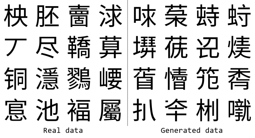
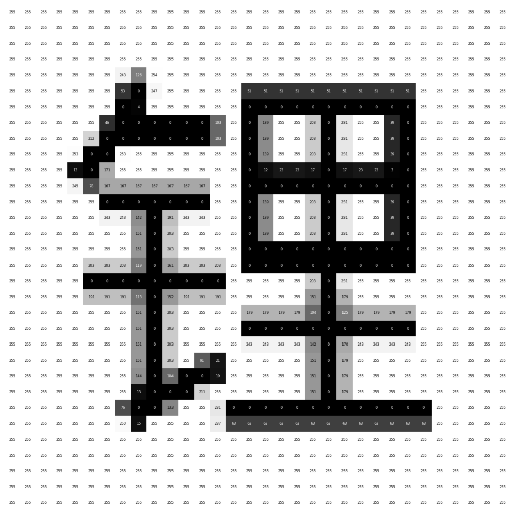
The examples will be based on the glyffuser, a minimal text-to-image diffusion model that I previously implemented and wrote about. The architecture of this model is a standard text-to-image denoising diffusion model without any bells or whistles. It was trained to generate pictures of new “Chinese” glyphs from English definitions. Have a look at the picture below — even if you’re not familiar with Chinese writing, I hope you’ll agree that the generated glyphs look pretty similar to the real ones!

What exactly is it that diffusion models learn?

Generative Ai models are often said to take a big pile of data and “learn” it. For text-to-image diffusion models, the data takes the form of pairs of images and descriptive text. But what exactly is it that we want the model to learn? First, let’s forget about the text for a moment and concentrate on what we are trying to generate: the images.

Probability distributions

Broadly, we can say that we want a generative AI model to learn the underlying probability distribution of the data. What does this mean? Consider the one-dimensional normal (Gaussian) distribution below, commonly written 𝒩(μ,σ²) and parameterized with mean μ = 0 and variance σ² = 1. The black curve below shows the probability density function. We can sample from it: drawing values such that over a large number of samples, the set of values reflects the underlying distribution. These days, we can simply write something like x = random.gauss(0, 1) in Python to sample from the standard normal distribution, although the computational sampling process itself is non-trivial!

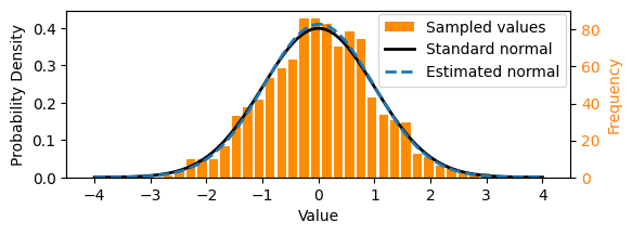
We could think of a set of numbers sampled from the above normal distribution as a simple dataset, like that shown as the orange histogram above. In this particular case, we can calculate the parameters of the underlying distribution using maximum likelihood estimation, i.e. by working out the mean and variance. The normal distribution estimated from the samples is shown by the dotted line above. To take some liberties with terminology, you might consider this as a simple example of “learning” an underlying probability distribution. We can also say that here we explicitly learnt the distribution, in contrast with the implicit methods that diffusion models use.

Conceptually, this is all that generative AI is doing — learning a distribution, then sampling from that distribution!

Data representations

What, then, does the underlying probability distribution of a more complex dataset look like, such as that of the image dataset we want to use to train our diffusion model?

First, we need to know what the representation of the data is. Generally, a machine learning (ML) model requires data inputs with a consistent representation, i.e. format. For the example above, it was simply numbers (scalars). For images, this representation is commonly a fixed-length vector.

The image dataset used for the glyffuser model is ~21,000 pictures of Chinese glyphs. The images are all the same size, 128 × 128 = 16384 pixels, and greyscale (single-channel color). Thus an obvious choice for the representation is a vector x of length 16384, where each element corresponds to the color of one pixel: x = (x₁,x₂,…,x₁₆₃₈₄). We can call the domain of all possible images for our dataset “pixel space”.

Dataset visualization

We make the assumption that our individual data samples, x, are actually sampled from an underlying probability distribution, q(x), in pixel space, much as the samples from our first example were sampled from an underlying normal distribution in 1-dimensional space. Note: the notation x ∼ q(x) is commonly used to mean: “the random variable x sampled from the probability distribution q(x).”

This distribution is clearly much more complex than a Gaussian and cannot be easily parameterized — we need to learn it with a ML model, which we’ll discuss later. First, let’s try to visualize the distribution to gain a better intution.

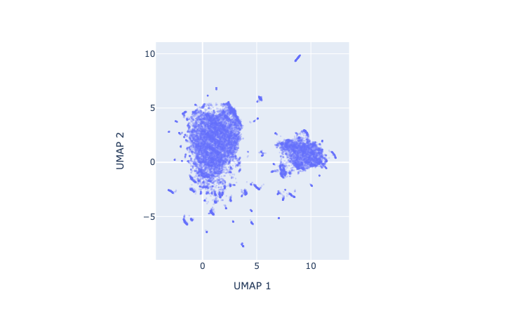
As humans find it difficult to see in more than 3 dimensions, we need to reduce the dimensionality of our data. A small digression on why this works: the manifold hypothesis posits that natural datasets lie on lower dimensional manifolds embedded in a higher dimensional space — think of a line embedded in a 2-D plane, or a plane embedded in 3-D space. We can use a dimensionality reduction technique such as UMAP to project our dataset from 16384 to 2 dimensions. The 2-D projection retains a lot of structure, consistent with the idea that our data lie on a lower dimensional manifold embedded in pixel space. In our UMAP, we see two large clusters corresponding to characters in which the components are arranged either horizontally (e.g. 明) or vertically (e.g. 草). An interactive version of the plot below with popups on each datapoint is linked here.

Let’s now use this low-dimensional UMAP dataset as a visual shorthand for our high-dimensional dataset. Remember, we assume that these individual points have been sampled from a continuous underlying probability distribution q(x). To get a sense of what this distribution might look like, we can apply a KDE (kernel density estimation) over the UMAP dataset. (Note: this is just an approximation for visualization purposes.)

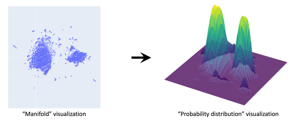
This gives a sense of what q(x) should look like: clusters of glyphs correspond to high-probability regions of the distribution. The true q(x) lies in 16384 dimensions — this is the distribution we want to learn with our diffusion model.

We showed that for a simple distribution such as the 1-D Gaussian, we could calculate the parameters (mean and variance) from our data. However, for complex distributions such as images, we need to call on ML methods. Moreover, what we will find is that for diffusion models in practice, rather than parameterizing the distribution directly, they learn it implicitly through the process of learning how to transform noise into data over many steps.

Takeaway

The aim of generative AI such as diffusion models is to learn the complex probability distributions underlying their training data and then sample from these distributions.

How and why do diffusion models work?

Diffusion models have recently come into the spotlight as a particularly effective method for learning these probability distributions. They generate convincing images by starting from pure noise and gradually refining it. To whet your interest, have a look at the animation below that shows the denoising process generating 16 samples.

In this section we’ll only talk about the mechanics of how these models work but if you’re interested in how they arose from the broader context of generative models, have a look at the further reading section below.

What is “noise”?

Let’s first precisely define noise, since the term is thrown around a lot in the context of diffusion. In particular, we are talking about Gaussian noise: consider the samples we talked about in the section about probability distributions. You could think of each sample as an image of a single pixel of noise. An image that is “pure Gaussian noise”, then, is one in which each pixel value is sampled from an independent standard Gaussian distribution, 𝒩(0,1). For a pure noise image in the domain of our glyph dataset, this would be noise drawn from 16384 separate Gaussian distributions. You can see this in the previous animation. One thing to keep in mind is that we can choose the means of these noise distributions, i.e. center them, on specific values — the pixel values of an image, for instance.

For convenience, you’ll often find the noise distributions for image datasets written as a single multivariate distribution 𝒩(0,I) where I is the identity matrix, a covariance matrix with all diagonal entries equal to 1 and zeroes elsewhere. This is simply a compact notation for a set of multiple independent Gaussians — i.e. there are no correlations between the noise on different pixels. In the basic implementations of diffusion models, only uncorrelated (a.k.a. “isotropic”) noise is used. This article contains an excellent interactive introduction on multivariate Gaussians.

Diffusion process overview

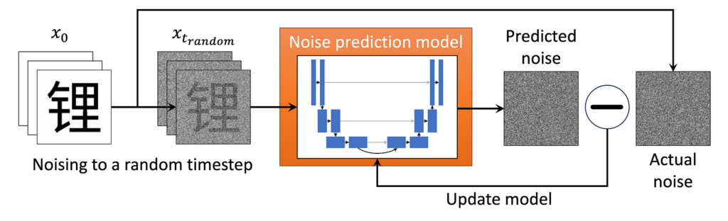
Below is an adaptation of the somewhat-famous diagram from Ho et al.’s seminal paper “Denoising Diffusion Probabilistic Models” which gives an overview of the whole diffusion process:

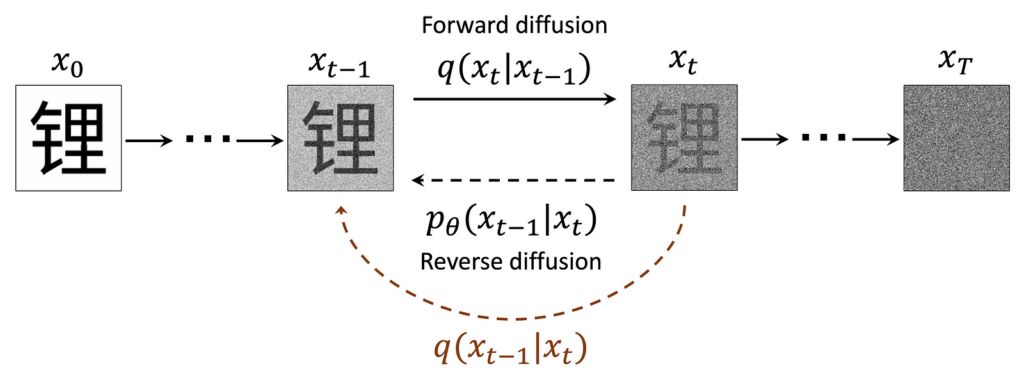
I found that there was a lot to unpack in this diagram and simply understanding what each component meant was very helpful, so let’s go through it and define everything step by step.

We previously used x ∼ q(x) to refer to our data. Here, we’ve added a subscript, xₜ, to denote timestep t indicating how many steps of “noising” have taken place. We refer to the samples noised a given timestep as x ∼ q(xₜ). x₀​ is clean data and xₜ (t = T) ∼ 𝒩(0,1) is pure noise.

We define a forward diffusion process whereby we corrupt samples with noise. This process is described by the distribution q(xₜ|xₜ₋₁). If we could access the hypothetical reverse process q(xₜ₋₁|xₜ), we could generate samples from noise. As we cannot access it directly because we would need to know x₀​, we use ML to learn the parameters, θ, of a model of this process, 𝑝θ(𝑥ₜ₋₁∣𝑥ₜ). (That should be p subscript θ but medium cannot render it.)

In the following sections we go into detail on how the forward and reverse diffusion processes work.

Forward diffusion, or “noising”

Used as a verb, “noising” an image refers to applying a transformation that moves it towards pure noise by scaling down its pixel values toward 0 while adding proportional Gaussian noise. Mathematically, this transformation is a multivariate Gaussian distribution centered on the pixel values of the preceding image.

In the forward diffusion process, this noising distribution is written as q(xₜ|xₜ₋₁) where the vertical bar symbol “|” is read as “given” or “conditional on”, to indicate the pixel means are passed forward from q(xₜ₋₁) At t = T where T is a large number (commonly 1000) we aim to end up with images of pure noise (which, somewhat confusingly, is also a Gaussian distribution, as discussed previously).

The marginal distributions q(xₜ) represent the distributions that have accumulated the effects of all the previous noising steps (marginalization refers to integration over all possible conditions, which recovers the unconditioned distribution).

Since the conditional distributions are Gaussian, what about their variances? They are determined by a variance schedule that maps timesteps to variance values. Initially, an empirically determined schedule of linearly increasing values from 0.0001 to 0.02 over 1000 steps was presented in Ho et al. Later research by Nichol & Dhariwal suggested an improved cosine schedule. They state that a schedule is most effective when the rate of information destruction through noising is relatively even per step throughout the whole noising process.

Forward diffusion intuition

As we encounter Gaussian distributions both as pure noise q(xₜ, t = T) and as the noising distribution q(xₜ|xₜ₋₁), I’ll try to draw the distinction by giving a visual intuition of the distribution for a single noising step, q(x₁∣x₀), for some arbitrary, structured 2-dimensional data:

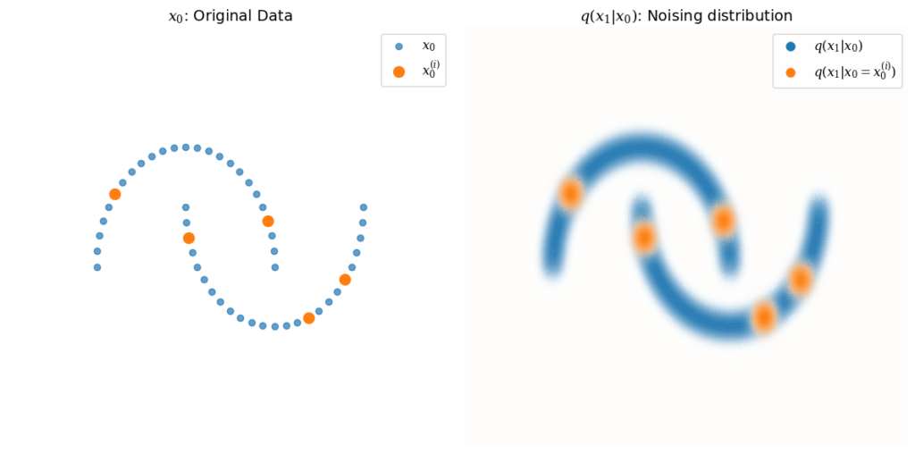
The distribution q(x₁∣x₀) is Gaussian, centered around each point in x₀, shown in blue. Several example points x₀⁽ⁱ⁾ are picked to illustrate this, with q(x₁∣x₀ = x₀⁽ⁱ⁾) shown in orange.

In practice, the main usage of these distributions is to generate specific instances of noised samples for training (discussed further below). We can calculate the parameters of the noising distributions at any timestep t directly from the variance schedule, as the chain of Gaussians is itself also Gaussian. This is very convenient, as we don’t need to perform noising sequentially—for any given starting data x₀⁽ⁱ⁾, we can calculate the noised sample xₜ⁽ⁱ⁾ by sampling from q(xₜ∣x₀ = x₀⁽ⁱ⁾) directly.

Forward diffusion visualization

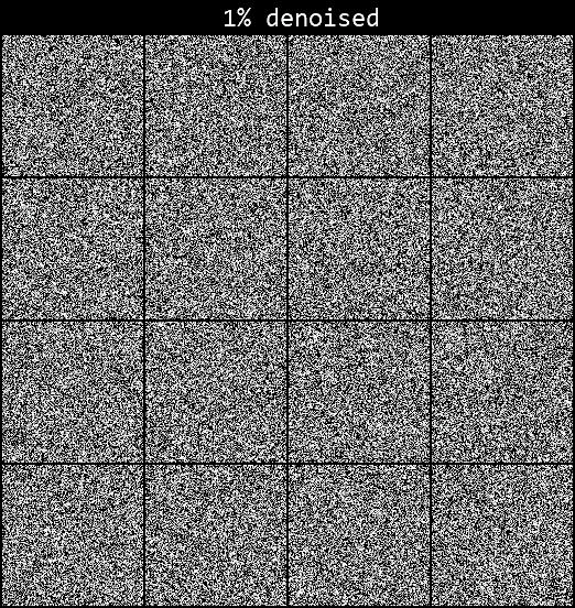
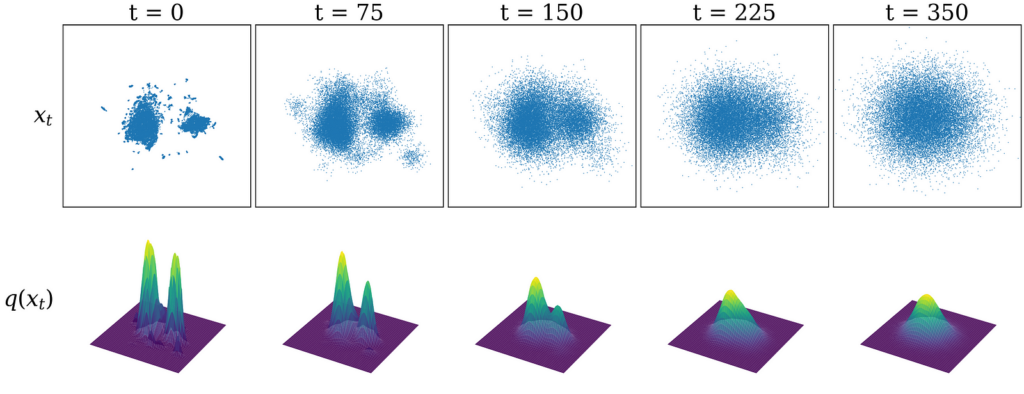
Let’s now return to our glyph dataset (once again using the UMAP visualization as a visual shorthand). The top row of the figure below shows our dataset sampled from distributions noised to various timesteps: xₜ ∼ q(xₜ). As we increase the number of noising steps, you can see that the dataset begins to resemble pure Gaussian noise. The bottom row visualizes the underlying probability distribution q(xₜ).

Reverse diffusion overview

It follows that if we knew the reverse distributions q(xₜ₋₁∣xₜ), we could repeatedly subtract a small amount of noise, starting from a pure noise sample xₜ at t = T to arrive at a data sample x₀ ∼ q(x₀). In practice, however, we cannot access these distributions without knowing x₀ beforehand. Intuitively, it’s easy to make a known image much noisier, but given a very noisy image, it’s much harder to guess what the original image was.

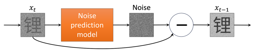
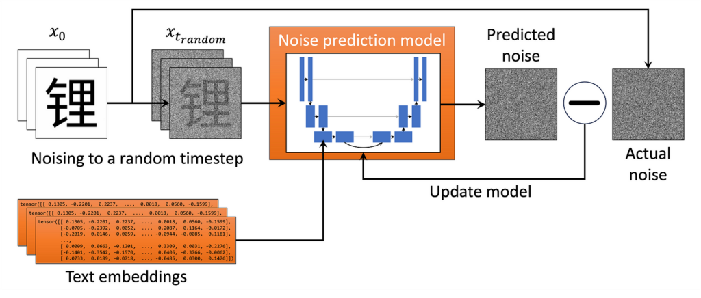
So what are we to do? Since we have a large amount of data, we can train an ML model to accurately guess the original image that any given noisy image came from. Specifically, we learn the parameters θ of an ML model that approximates the reverse noising distributions, pθ(xₜ₋₁ ∣ xₜ) for t = 0, …, T. In practice, this is embodied in a single noise prediction model trained over many different samples and timesteps. This allows it to denoise any given input, as shown in the figure below.

Next, let’s go over how this noise prediction model is implemented and trained in practice.

How the model is implemented

First, we define the ML model — generally a deep neural network of some sort — that will act as our noise prediction model. This is what does the heavy lifting! In practice, any ML model that inputs and outputs data of the correct size can be used; the U-net, an architecture particularly suited to learning images, is what we use here and frequently chosen in practice. More recent models also use vision transformers.

Then we run the training loop depicted in the figure above:

• We take a random image from our dataset and noise it to a random timestep tt. (In practice, we speed things up by doing many examples in parallel!)
• We feed the noised image into the ML model and train it to predict the (known to us) noise in the image. We also perform timestep conditioning by feeding the model a timestep embedding, a high-dimensional unique representation of the timestep, so that the model can distinguish between timesteps. This can be a vector the same size as our image directly added to the input (see here for a discussion of how this is implemented).
• The model “learns” by minimizing the value of a loss function, some measure of the difference between the predicted and actual noise. The mean square error (the mean of the squares of the pixel-wise difference between the predicted and actual noise) is used in our case.
• Repeat until the model is well trained.

Note: A neural network is essentially a function with a huge number of parameters (on the order of 10⁶ for the glyffuser). Neural network ML models are trained by iteratively updating their parameters using backpropagation to minimize a given loss function over many training data examples. This is an excellent introduction. These parameters effectively store the network’s “knowledge”.

A noise prediction model trained in this way eventually sees many different combinations of timesteps and data examples. The glyffuser, for example, was trained over 100 epochs (runs through the whole data set), so it saw around 2 million data samples. Through this process, the model implicity learns the reverse diffusion distributions over the entire dataset at all different timesteps. This allows the model to sample the underlying distribution q(x₀) by stepwise denoising starting from pure noise. Put another way, given an image noised to any given level, the model can predict how to reduce the noise based on its guess of what the original image. By doing this repeatedly, updating its guess of the original image each time, the model can transform any noise to a sample that lies in a high-probability region of the underlying data distribution.

Reverse diffusion in practice

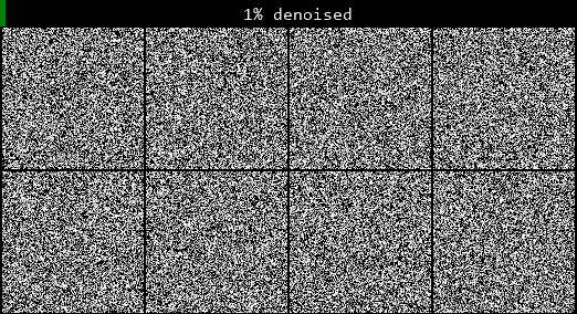
We can now revisit this video of the glyffuser denoising process. Recall a large number of steps from sample to noise e.g. T = 1000 is used during training to make the noise-to-sample trajectory very easy for the model to learn, as changes between steps will be small. Does that mean we need to run 1000 denoising steps every time we want to generate a sample?

Luckily, this is not the case. Essentially, we can run the single-step noise prediction but then rescale it to any given step, although it might not be very good if the gap is too large! This allows us to approximate the full sampling trajectory with fewer steps. The video above uses 120 steps, for instance (most implementations will allow the user to set the number of sampling steps).

Recall that predicting the noise at a given step is equivalent to predicting the original image x₀, and that we can access the equation for any noised image deterministically using only the variance schedule and x₀. Thus, we can calculate xₜ₋ₖ based on any denoising step. The closer the steps are, the better the approximation will be.

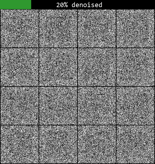
Too few steps, however, and the results become worse as the steps become too large for the model to effectively approximate the denoising trajectory. If we only use 5 sampling steps, for example, the sampled characters don’t look very convincing at all:

There is then a whole literature on more advanced sampling methods beyond what we’ve discussed so far, allowing effective sampling with much fewer steps. These often reframe the sampling as a differential equation to be solved deterministically, giving an eerie quality to the sampling videos — I’ve included one at the end if you’re interested. In production-level models, these are usually preferred over the simple method discussed here, but the basic principle of deducing the noise-to-sample trajectory is the same. A full discussion is beyond the scope of this article but see e.g. this paper and its corresponding implementation in the Hugging Face diffusers library for more information.

Alternative intuition from score function

To me, it was still not 100% clear why training the model on noise prediction generalises so well. I found that an alternative interpretation of diffusion models known as “score-based modeling” filled some of the gaps in intuition (for more information, refer to Yang Song’s definitive article on the topic.)

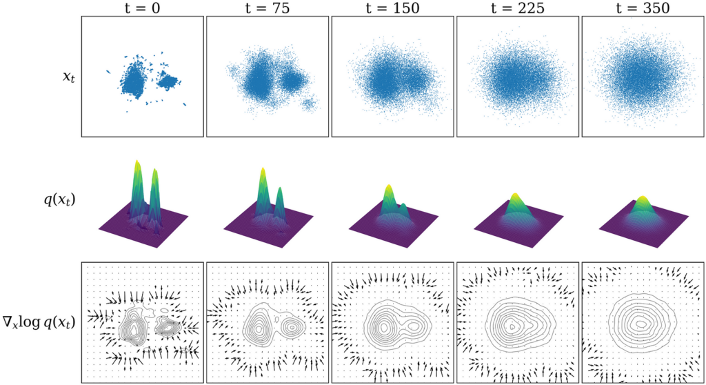
I try to give a visual intuition in the bottom row of the figure above: essentially, learning the noise in our diffusion model is equivalent (to a constant factor) to learning the score function, which is the gradient of the log of the probability distribution: ∇ₓ log q(x). As a gradient, the score function represents a vector field with vectors pointing towards the regions of highest probability density. Subtracting the noise at each step is then equivalent to moving following the directions in this vector field towards regions of high probability density.

As long as there is some signal, the score function effectively guides sampling, but in regions of low probability it tends towards zero as there is little to no gradient to follow. Using many steps to cover different noise levels allows us to avoid this, as we smear out the gradient field at high noise levels, allowing sampling to converge even if we start from low probability density regions of the distribution. The figure shows that as the noise level is increased, more of the domain is covered by the score function vector field.

Summary

• The aim of diffusion models is learn the underlying probability distribution of a dataset and then be able to sample from it. This requires forward and reverse diffusion (noising) processes.
• The forward noising process takes samples from our dataset and gradually adds Gaussian noise (pushes them off the data manifold). This forward process is computationally efficient because any level of noise can be added in closed form a single step.
• The reverse noising process is challenging because we need to predict how to remove the noise at each step without knowing the original data point in advance. We train a ML model to do this by giving it many examples of data noised at different timesteps.
• Using very small steps in the forward noising process makes it easier for the model to learn to reverse these steps, as the changes are small.
• By applying the reverse noising process iteratively, the model refines noisy samples step by step, eventually producing a realistic data point (one that lies on the data manifold).

Takeaway

Diffusion models are a powerful framework for learning complex data distributions. The distributions are learnt implicitly by modelling a sequential denoising process. This process can then be used to generate samples similar to those in the training distribution.

Once you’ve trained a model, how do you get useful stuff out of it?

Earlier uses of generative AI such as “This Person Does Not Exist” (ca. 2019) made waves simply because it was the first time most people had seen AI-generated photorealistic human faces. A generative adversarial network or “GAN” was used in that case, but the principle remains the same: the model implicitly learnt a underlying data distribution — in that case, human faces — then sampled from it. So far, our glyffuser model does a similar thing: it samples randomly from the distribution of Chinese glyphs.

The question then arises: can we do something more useful than just sample randomly? You’ve likely already encountered text-to-image models such as Dall-E. They are able to incorporate extra meaning from text prompts into the diffusion process — this in known as conditioning. Likewise, diffusion models for scientific scientific applications like protein (e.g. Chroma, RFdiffusion, AlphaFold3) or inorganic crystal structure generation (e.g. MatterGen) become much more useful if can be conditioned to generate samples with desirable properties such as a specific symmetry, bulk modulus, or band gap.

Conditional distributions

We can consider conditioning as a way to guide the diffusion sampling process towards particular regions of our probability distribution. We mentioned conditional distributions in the context of forward diffusion. Below we show how conditioning can be thought of as reshaping a base distribution.

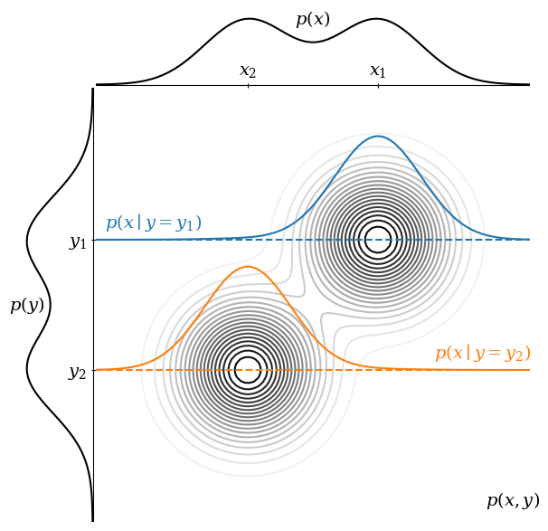
Consider the figure above. Think of p(x) as a distribution we want to sample from (i.e., the images) and p(y) as conditioning information (i.e., the text dataset). These are the marginal distributions of a joint distribution p(x, y). Integrating p(x, y) over y recovers p(x), and vice versa.

Sampling from p(x), we are equally likely to get x₁ or x₂. However, we can condition on p(y = y₁) to obtain p(x∣y = y₁). You can think of this as taking a slice through p(x, y) at a given value of y. In this conditioned distribution, we are much more likely to sample at x₁ than x₂.

In practice, in order to condition on a text dataset, we need to convert the text into a numerical form. We can do this using large language model (LLM) embeddings that can be injected into the noise prediction model during training.

Embedding text with an LLM

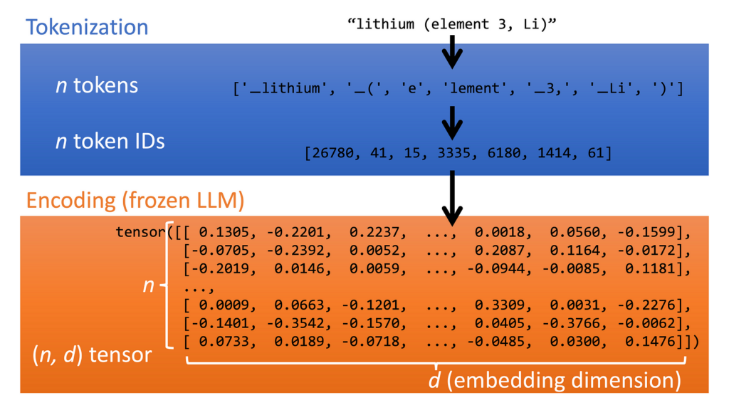
In the glyffuser, our conditioning information is in the form of English text definitions. We have two requirements: 1) ML models prefer fixed-length vectors as input. 2) The numerical representation of our text must understand context — if we have the words “lithium” and “element” nearby, the meaning of “element” should be understood as “chemical element” rather than “heating element”. Both of these requirements can be met by using a pre-trained LLM.

The diagram below shows how an LLM converts text into fixed-length vectors. The text is first tokenized (LLMs break text into tokens, small chunks of characters, as their basic unit of interaction). Each token is converted into a base embedding, which is a fixed-length vector of the size of the LLM input. These vectors are then passed through the pre-trained LLM (here we use the encoder portion of Google’s T5 model), where they are imbued with additional contextual meaning. We end up with a array of n vectors of the same length d, i.e. a (n, d) sized tensor.

Note: in some models, notably Dall-E, additional image-text alignment is performed using contrastive pretraining. Imagen seems to show that we can get away without doing this.

Training the diffusion model with text conditioning

The exact method that this embedding vector is injected into the model can vary. In Google’s Imagen model, for example, the embedding tensor is pooled (combined into a single vector in the embedding dimension) and added into the data as it passes through the noise prediction model; it is also included in a different way using cross-attention (a method of learning contextual information between sequences of tokens, most famously used in the transformer models that form the basis of LLMs like ChatGPT).

In the glyffuser, we only use cross-attention to introduce this conditioning information. While a significant architectural change is required to introduce this additional information into the model, the loss function for our noise prediction model remains exactly the same.

Testing the conditioned diffusion model

Let’s do a simple test of the fully trained conditioned diffusion model. In the figure below, we try to denoise in a single step with the text prompt “Gold”. As touched upon in our interactive UMAP, Chinese characters often contain components known as radicals which can convey sound (phonetic radicals) or meaning (semantic radicals). A common semantic radical is derived from the character meaning “gold”, “金”, and is used in characters that are in some broad sense associated with gold or metals.

The figure shows that even though a single step is insufficient to approximate the denoising trajectory very well, we have moved into a region of our probability distribution with the “金” radical. This indicates that the text prompt is effectively guiding our sampling towards a region of the glyph probability distribution related to the meaning of the prompt. The animation below shows a 120 step denoising sequence for the same prompt, “Gold”. You can see that every generated glyph has either the 釒 or 钅 radical (the same radical in traditional and simplified Chinese, respectively).

Takeaway

Conditioning enables us to sample meaningful outputs from diffusion models.

Further remarks

I found that with the help of tutorials and existing libraries, it was possible to implement a working diffusion model despite not having a full understanding of what was going on under the hood. I think this is a good way to start learning and highly recommend Hugging Face’s tutorial on training a simple diffusion model using their diffusers Python library (which now includes my small bugfix!).

I’ve omitted some topics that are crucial to how production-grade diffusion models function, but are unnecessary for core understanding. One is the question of how to generate high resolution images. In our example, we did everything in pixel space, but this becomes very computationally expensive for large images. The general approach is to perform diffusion in a smaller space, then upscale it in a separate step. Methods include latent diffusion (used in Stable Diffusion) and cascaded super-resolution models (used in Imagen). Another topic is classifier-free guidance, a very elegant method for boosting the conditioning effect to give much better prompt adherence. I show the implementation in my previous post on the glyffuser and highly recommend this article if you want to learn more.

Further reading

A non-exhaustive list of materials I found very helpful:

Fun extras

Diffusion sampling using the DPMSolverSDEScheduler developed by Katherine Crowson and implemented in Hugging Face diffusers—note the smooth transition from noise to data.