What if you want to write the whole object detection training pipeline from scratch, so you can understand each step and be able to customize it? That’s what I set out to do. I examined several well-known object detection pipelines and designed one that best suits my needs and tasks. Thanks to Ultralytics, YOLOx, DAMO-YOLO, RT-DETR and D-FINE repos, I leveraged them to gain deeper understanding into various design details. I ended up implementing SoTA real-time object detection model D-FINE in my custom pipeline.
Plan
- Dataset, Augmentations and transforms:
- Mosaic (with affine transforms)
- Mixup and Cutout
- Other augmentations with bounding boxes
- Letterbox vs simple resize
- Training:
- Optimizer
- Scheduler
- EMA
- Batch accumulation
- AMP
- Grad clipping
- Logging
- Metrics:
- mAPs from TorchMetrics / cocotools
- How to compute Precision, Recall, IoU?
- Pick a suitable solution for your case
- Experiments
- Attention to data preprocessing
- Where to start
Dataset
Dataset processing is the first thing you usually start working on. With object detection, you need to load your image and annotations. Annotations are often stored in COCO format as a json file or YOLO format, with txt file for each image. Let’s take a look at the YOLO format: Each line is structured as: class_id, x_center, y_center, width, height, where bbox values are normalized between 0 and 1.
When you have your images and txt files, you can write your dataset class, nothing tricky here. Load everything, transform (augmentations included) and return during training. I prefer splitting the data by creating a CSV file for each split and then reading it in the Dataloader class rather than physically moving files into train/val/test folders. This is an example of a customization that helped my use case.
Augmentations
Firstly, when augmenting images for object detection, it’s crucial to apply the same transformations to the bounding boxes. To comfortably do that I use Albumentations lib. For example:
    def _init_augs(self, cfg) -> None:
        if self.keep_ratio:
            resize = [
                A.LongestMaxSize(max_size=max(self.target_h, self.target_w)),
                A.PadIfNeeded(
                    min_height=self.target_h,
                    min_width=self.target_w,
                    border_mode=cv2.BORDER_CONSTANT,
                    fill=(114, 114, 114),
                ),
            ]

        else:
            resize = [A.Resize(self.target_h, self.target_w)]
        norm = [
            A.Normalize(mean=self.norm[0], std=self.norm[1]),
            ToTensorV2(),
        ]

        if self.mode == "train":
            augs = [
                A.RandomBrightnessContrast(p=cfg.train.augs.brightness),
                A.RandomGamma(p=cfg.train.augs.gamma),
                A.Blur(p=cfg.train.augs.blur),
                A.GaussNoise(p=cfg.train.augs.noise, std_range=(0.1, 0.2)),
                A.ToGray(p=cfg.train.augs.to_gray),
                A.Affine(
                    rotate=[90, 90],
                    p=cfg.train.augs.rotate_90,
                    fit_output=True,
                ),
                A.HorizontalFlip(p=cfg.train.augs.left_right_flip),
                A.VerticalFlip(p=cfg.train.augs.up_down_flip),
            ]

            self.transform = A.Compose(
                augs + resize + norm,
                bbox_params=A.BboxParams(format="pascal_voc", label_fields=["class_labels"]),
            )

        elif self.mode in ["val", "test", "bench"]:
            self.mosaic_prob = 0
            self.transform = A.Compose(
                resize + norm,
                bbox_params=A.BboxParams(format="pascal_voc", label_fields=["class_labels"]),
            )
Secondly, there are a lot of interesting and not trivial augmentations:
- Mosaic. The idea is simple, let’s take several images (for example 4), and stack them together in a grid (2×2). Then let’s do some affine transforms and feed it to the model.
- MixUp. Originally used in image classification (it’s surprising that it works). Idea – let’s take two images, put them onto each other with some percent of transparency. In classification models it usually means that if one image is 20% transparent and the second is 80%, then the model should predict 80% for class 1 and 20% for class 2. In object detection we just get more objects into 1 image.
- Cutout. Cutout involves removing parts of the image (by replacing them with black pixels) to help the model learn more robust features.
I see mosaic often applied with Probability 1.0 of the first ~90% of epochs. Then, it’s usually turned off, and lighter augmentations are used. The same idea applies to mixup, but I see it being used a lot less (for the most popular detection framework, Ultralytics, it’s turned off by default. For another one, I see P=0.15). Cutout seems to be used less frequently.
You can read more about those augmentations in these two articles: 1, 2.
Results from just turning on mosaic are pretty good (darker one without mosaic got mAP 0.89 vs 0.92 with, tested on a real dataset)
Letterbox or simple resize?
During training, you usually resize the input image to a square. Models often use 640×640 and benchmark on COCO dataset. And there are two main ways how you get there:
- Simple resize to a target size.
- Letterbox: Resize the longest side to the target size (e.g., 640), preserving the aspect ratio, and pad the shorter side to reach the target dimensions.
Both approaches have advantages and disadvantages. Let’s discuss them first, and then I will share the results of numerous experiments I ran comparing these approaches.
Simple resize:
- Compute goes to the whole image, with no useless padding.
- “Dynamic” aspect ratio may act as a form of regularization.
- Inference preprocessing perfectly matches training preprocessing (augmentations excluded).
- Kills real geometry. Resize distortion could affect the spatial relationships in the image. Although it might be a human bias to think that a fixed aspect ratio is important.
Letterbox:
- Preserves real aspect ratio.
- During inference, you can cut padding and run not on the square image if you don’t lose accuracy (some models can degrade).
- Can train on a bigger image size, then inference with cut padding to get the same inference latency as with simple resize. For example 640×640 vs 832×480. The second one will preserve the aspect ratios and objects will appear +- the same size.
- Part of the compute is wasted on gray padding.
- Objects get smaller.
How to test it and decide which one to use?
Train from scratch with parameters:
- Simple resize, 640×640
- Keep aspect ratio, max side 640, and add padding (as a baseline)
- Keep aspect ratio, larger image size (for example max side 832), and add padding Then inference 3 models. When the aspect ratio is preserved – cut padding during the inference. Compare latency and metrics.
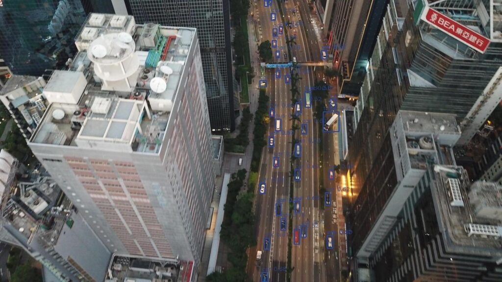
Example of the same image from above with cut padding (640 × 384):
Here is what happens when you preserve ratio and inference by cutting gray padding:
params                  |   F1 score  |  latency (ms).   |
-------------------------+-------------+-----------------|
ratio kept, 832         |    0.633    |        33.5      |
no ratio, 640x640       |    0.617    |        33.4      |
As shown, training with preserved aspect ratio at a larger size (832) achieved a higher F1 score (0.633) compared to a simple 640×640 resize (F1 score of 0.617), while the latency remained similar. Note that some models may degrade if the padding is removed during inference, which kills the whole purpose of this trick and probably the letterbox too.
What does this mean:
Training from scratch:
- With the same image size, simple resize gets better accuracy than letterbox.
- For letterbox, If you cut padding during the inference and your model doesn’t lose accuracy – you can train and inference with a bigger image size to match the latency, and get a little bit higher metrics (as in the example above).
Training with pre-trained weights initialized:
- If you finetune – use the same tactic as the pre-trained model did, it should give you the best results if the datasets are not too different.
For D-FINE I see lower metrics when cutting padding during inference. Also the model was pre-trained on a simple resize. For YOLO, a letterbox is typically a good choice.
Training
Every ML engineer should know how to implement a training loop. Although PyTorch does much of the heavy lifting, you might still feel overwhelmed by the number of design choices available. Here are some key components to consider:
- Optimizer – start with Adam/AdamW/SGD.
- Scheduler – fixed LR can be ok for Adams, but take a look at StepLR, CosineAnnealingLR or OneCycleLR.
- EMA. This is a nice technique that makes training smoother and sometimes achieves higher metrics. After each batch, you update a secondary model (often called the EMA model) by computing an exponential moving average of the primary model’s weights.
- Batch accumulation is nice when your vRAM is very limited. Training a transformer-based object detection model means that in some cases even in a middle-sized model you only can fit 4 images into the vRAM. By accumulating gradients over several batches before performing an optimizer step, you effectively simulate a larger batch size without exceeding your memory constraints. Another use case is when you have a lot of negatives (images without target objects) in your dataset and a small batch size, you can encounter unstable training. Batch accumulation can also help here.
- AMP uses half precision automatically where applicable. It reduces vRAM usage and makes training faster (if you have a GPU that supports it). I see 40% less vRAM usage and at least a 15% training speed increase.
- Grad clipping. Often, when you use AMP, training can become less stable. This can also happen with higher LRs. When your gradients are too big, training will fail. Gradient clipping will make sure gradients are never bigger than a certain value.
- Logging. Try Hydra for configs and something like Weights and Biases or Clear ML for experiment tracking. Also, log everything locally. Save your best weights, and metrics, so after numerous experiments, you can always find all the info on the model you need.
    def train(self) -> None:
        best_metric = 0
        cur_iter = 0
        ema_iter = 0
        one_epoch_time = None

        def optimizer_step(step_scheduler: bool):
            """
            Clip grads, optimizer step, scheduler step, zero grad, EMA model update
            """
            nonlocal ema_iter
            if self.amp_enabled:
                if self.clip_max_norm:
                    self.scaler.unscale_(self.optimizer)

torch.nn.utils.clip_grad_norm_(self.model.parameters(), self.clip_max_norm)
                self.scaler.step(self.optimizer)
                self.scaler.update()

            else:
                if self.clip_max_norm:

torch.nn.utils.clip_grad_norm_(self.model.parameters(), self.clip_max_norm)
                self.optimizer.step()

            if step_scheduler:
                self.scheduler.step()
            self.optimizer.zero_grad()

            if self.ema_model:
                ema_iter += 1
                self.ema_model.update(ema_iter, self.model)

        for epoch in range(1, self.epochs + 1):
            epoch_start_time = time.time()
            self.model.train()
            self.loss_fn.train()
            losses = []

            with tqdm(self.train_loader, unit="batch") as tepoch:
                for batch_idx, (inputs, targets, _) in enumerate(tepoch):
                    tepoch.set_description(f"Epoch {epoch}/{self.epochs}")
                    if inputs is None:
                        continue
                    cur_iter += 1

                    inputs = inputs.to(self.device)
                    targets = [
                        {
                            k: (v.to(self.device) if (v is not None and hasattr(v, "to")) else v)
                            for k, v in t.items()
                        }
                        for t in targets
                    ]

                    lr = self.optimizer.param_groups[0]["lr"]

                    if self.amp_enabled:
                        with autocast(self.device, cache_enabled=True):
                            output = self.model(inputs, targets=targets)
                        with autocast(self.device, enabled=False):
                            loss_dict = self.loss_fn(output, targets)
                        loss = sum(loss_dict.values()) / self.b_accum_steps
                        self.scaler.scale(loss).backward()

                    else:
                        output = self.model(inputs, targets=targets)
                        loss_dict = self.loss_fn(output, targets)
                        loss = sum(loss_dict.values()) / self.b_accum_steps
                        loss.backward()

                    if (batch_idx + 1) % self.b_accum_steps == 0:
                        optimizer_step(step_scheduler=True)

                    losses.append(loss.item())

                    tepoch.set_postfix(
                        loss=np.mean(losses) * self.b_accum_steps,
                        eta=calculate_remaining_time(
                            one_epoch_time,
                            epoch_start_time,
                            epoch,
                            self.epochs,
                            cur_iter,
                            len(self.train_loader),
                        ),
                        vram=f"{get_vram_usage()}%",
                    )

            # Final update for any leftover gradients from an incomplete accumulation step
            if (batch_idx + 1) % self.b_accum_steps != 0:
                optimizer_step(step_scheduler=False)

            wandb.log({"lr": lr, "epoch": epoch})

            metrics = self.evaluate(
                val_loader=self.val_loader,
                conf_thresh=self.conf_thresh,
                iou_thresh=self.iou_thresh,
                path_to_save=None,
            )

            best_metric = self.save_model(metrics, best_metric)
            save_metrics(
                {}, metrics, np.mean(losses) * self.b_accum_steps, epoch, path_to_save=None
            )

            if (
                epoch >= self.epochs - self.no_mosaic_epochs
                and self.train_loader.dataset.mosaic_prob
            ):
                self.train_loader.dataset.close_mosaic()

            if epoch == self.ignore_background_epochs:
                self.train_loader.dataset.ignore_background = False
                logger.info("Including background images")

            one_epoch_time = time.time() - epoch_start_time
Metrics
For object detection everyone uses mAP, and it is already standardized how we measure those. Use pycocotools or faster-coco-eval or TorchMetrics for mAP. But mAP means that we check how good the model is overall, on all confidence levels. mAP0.5 means that IoU threshold is 0.5 (everything lower is considered as a wrong prediction). I personally don’t fully like this metric, as in production we always use 1 confidence threshold. So why not set the threshold and then compute metrics? That’s why I also always calculate confusion matrices, and based on that – Precision, Recall, F1-score, and IoU.
But logic also might be tricky. Here is what I use:
- 1 GT (ground truth) object = 1 predicted object, and it’s a TP if IoU > threshold. If there is no prediction for a GT object – it’s a FN. If there is no GT for a prediction – it’s a FP.
- 1 GT should be matched by a prediction only 1 time. If there are 2 predictions for 1 GT, then I calculate 1 TP and 1 FP.
- Class ids should also match. If the model predicts class_0 but GT is class_1, it means FP += 1 and FN += 1.
During training, I select the best model based on the metrics that are relevant to the task. I typically consider the average of mAP50 and F1-score.
Model and loss
I haven’t discussed model architecture and loss function here. They usually go together, and you can choose any model you like and integrate it into your pipeline with everything from above. I did that with DAMO-YOLO and D-FINE, and the results were great.
Pick a suitable solution for your case
Many people use Ultralytics, however it has GPLv3, and you can’t use it in commercial projects unless your code is open source. So people often look into Apache 2 and MIT licensed models. Check out D-FINE, RT-DETR2 or some yolo models like Yolov9.
What if you want to customize something in the pipeline? When you build everything from scratch, you should have full control. Otherwise, try choosing a project with a smaller codebase, as a large one can make it difficult to isolate and modify individual components.
If you don’t need anything custom and your usage is allowed by the Ultralytics license – it’s a great repo to use, as it supports multiple tasks (classification, detection, instance segmentation, key points, oriented bounding boxes), models are efficient and achieve good scores. Reiterating ones more, you probably don’t need a custom training pipeline if you are not doing very specific things.
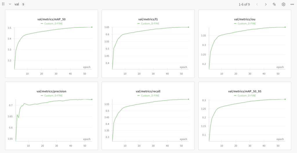
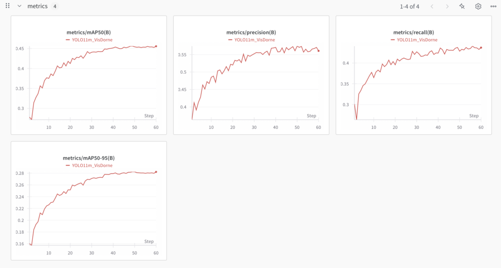
Experiments
Let me share some results I got with a custom training pipeline with the D-FINE model and compare it to the Ultralytics YOLO11 model on the VisDrone-DET2019 dataset.
Trained from scratch:
model                     |  mAP 0.50.   |    F1-score  |  Latency (ms)  |
---------------------------------+--------------+--------------+------------------|
YOLO11m TRT               |     0.417    |     0.568    |       15.6     |
YOLO11m TRT dynamic       |     -        |     0.568    |       13.3     |
YOLO11m OV                |      -       |     0.568    |      122.4     |
D-FINEm TRT               |    0.457     |     0.622    |       16.6     |
D-FINEm OV                |    0.457     |     0.622    |       115.3    |
From COCO pre-trained:
model          |    mAP 0.50   |   F1-score  |
------------------+------------|-------------|
YOLO11m        |     0.456     |    0.600    |
D-FINEm        |     0.506     |    0.649    |
Latency was measured on an RTX 3060 with TensorRT (TRT), static image size 640×640, including the time for cv2.imread. OpenVINO (OV) on i5 14000f (no iGPU). Dynamic means that during inference, gray padding is being cut for faster inference. It worked with the YOLO11 TensorRT version. More details about cutting gray padding above (Letterbox or simple resize section).
One disappointing result is the latency on intel N100 CPU with iGPU ($150 miniPC):
model            | Latency (ms) |
------------------+-------------|
YOLO11m          |       188    |
D-FINEm          |       272    |
D-FINEs          |       11     |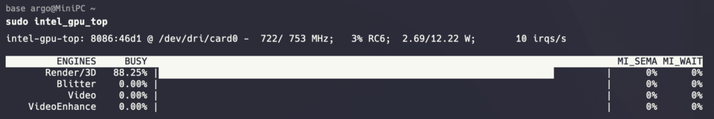
Here, traditional convolutional neural networks are noticeably faster, maybe because of optimizations in OpenVINO for GPUs.
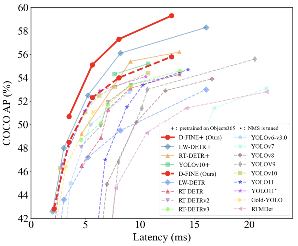
Overall, I conducted over 30 experiments with different datasets (including real-world datasets), models, and parameters and I can say that D-FINE gets better metrics. And it makes sense, as on COCO, it is also higher than all YOLO models.
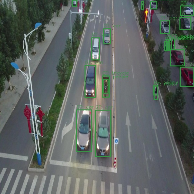
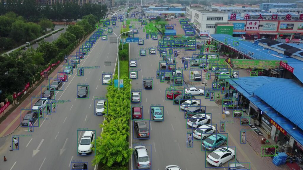
VisDrone experiments:
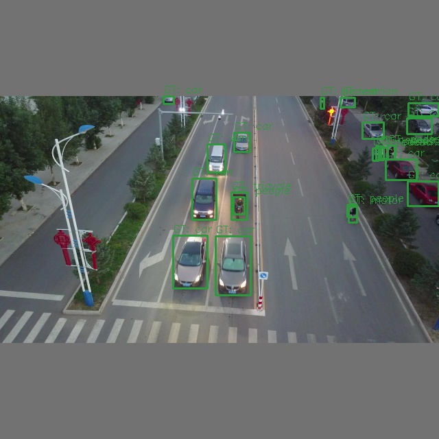
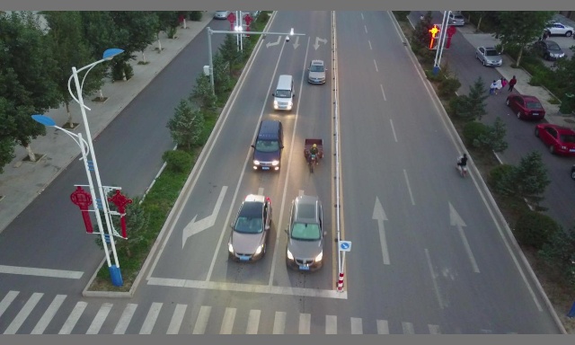
Example of D-FINE model predictions (green – GT, blue – pred):
Final results
Knowing all the details, let’s see a final comparison with the best settings for both models on i12400F and RTX 3060 with the VisDrone dataset:
model                              |   F1-score    |   Latency (ms)    |
-----------------------------------+---------------+-------------------|
YOLO11m TRT dynamic                |      0.600    |        13.3       |
YOLO11m OV                         |      0.600    |       122.4       |
D-FINEs TRT                        |      0.629    |        12.3       |
D-FINEs OV                         |      0.629    |        57.4       |
As shown above, I was able to use a smaller D-FINE model and achieve both faster inference time and accuracy than YOLO11. Beating Ultralytics, the most widely used real-time object detection model, in both speed and accuracy, is quite an accomplishment, isn’t it? The same pattern is observed across several other real-world datasets.
I also tried out YOLOv12, which came out while I was writing this article. It performed similarly to YOLO11 and even achieved slightly lower metrics (mAP 0.456 vs 0.452). It appears that YOLO models have been hitting the wall for the last couple of years. D-FINE was a great update for object detection models.
Finally, let’s see visually the difference between YOLO11m and D-FINEs. YOLO11m, conf 0.25, nms iou 0.5, latency 13.3ms:
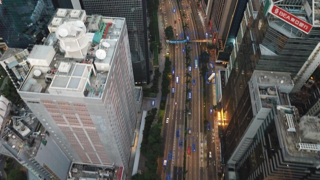
D-FINEs, conf 0.5, no nms, latency 12.3ms:
Both Precision and Recall are higher with the D-FINE model. And it’s also faster. Here is also “m” version of D-FINE:

Isn’t it crazy that even that one car on the left was detected?
Attention to data preprocessing
This part can go a little bit outside the scope of the article, but I want to at least quickly mention it, as some parts can be automated and used in the pipeline. What I definitely see as a Computer Vision engineer is that when engineers don’t spend time working with the data – they don’t get good models. You can have all SoTA models and everything done right, but garbage in – garbage out. So, I always pay a ton of attention to how to approach the task and how to gather, filter, validate, and annotate the data. Don’t think that the annotation team will do everything right. Get your hands dirty and check manually some portion of the dataset to be sure that annotations are good and collected images are representative.
Several quick ideas to look into:
- Remove duplicates and near duplicates from val/test sets. The model should not be validated on one sample two times, and definitely, you don’t want to have a data leak, by getting two same images, one in training and one in validation sets.
- Check how small your objects can be. Everything not visible to your eye should not be annotated. Also, remember that augmentations will make objects appear even smaller (for example, mosaic or zoom out). Configure these augmentations accordingly so you won’t end up with unusably small objects on the image.
- When you already have a model for a certain task and need more data – try using your model to pre-annotate new images. Check cases where the model fails and gather more similar cases.
Where to start
I worked a lot on this pipeline, and I am ready to share it with everyone who wants to try it out. It uses the SoTA D-FINE model under the hood and adds some features that were absent in the original repo (mosaic augmentations, batch accumulation, scheduler, more metrics, visualization of preprocessed images and eval predictions, exporting and inference code, better logging, unified and simplified configuration file).
Here is the link to my repo. Here is the original D-FINE repo, where I also contribute. If you need any help, please contact me on LinkedIn. Thank you for your time!
Citations and acknowledgments
@article{zhu2021detection,
  title={Detection and tracking meet drones challenge},
  author={Zhu, Pengfei and Wen, Longyin and Du, Dawei and Bian, Xiao and Fan, Heng and Hu, Qinghua and Ling, Haibin},
  journal={IEEE Transactions on Pattern Analysis and Machine Intelligence},
  volume={44},
  number={11},
  pages={7380--7399},
  year={2021},
  publisher={IEEE}
}@misc{peng2024dfine,
title={D-FINE: Redefine Regression Task in DETRs as Fine-grained Distribution Refinement},
author={Yansong Peng and Hebei Li and Peixi Wu and Yueyi Zhang and Xiaoyan Sun and Feng Wu},
year={2024},
eprint={2410.13842},
archivePrefix={arXiv},
primaryClass={cs.CV}
}