Stay Ahead, Stay ONMINE

Image Captioning, Transformer Mode On

Introduction In my previous article, I discussed one of the earliest Deep Learning approaches for image captioning. If you’re interested in reading it, you can find the link to that article at the end of this one. Today, I would like to talk about Image Captioning again, but this time with the more advanced neural network architecture. The deep learning I am going to talk about is the one proposed in the paper titled “CPTR: Full Transformer Network for Image Captioning,” written by Liu et al. back in 2021 [1]. Specifically, here I will reproduce the model proposed in the paper and explain the underlying theory behind the architecture. However, keep in mind that I won’t actually demonstrate the training process since I only want to focus on the model architecture. The idea behind CPTR In fact, the main idea of the CPTR architecture is exactly the same as the earlier image captioning model, as both use the encoder-decoder structure. Previously, in the paper titled “Show and Tell: A Neural Image Caption Generator” [2], the models used are GoogLeNet (a.k.a. Inception V1) and LSTM for the two components, respectively. The illustration of the model proposed in the Show and Tell paper is shown in the following figure. Figure 1. The neural network architecture for image captioning proposed in the Show and Tell paper [2]. Despite having the same encoder-decoder structure, what makes CPTR different from the previous approach is the basis of the encoder and the decoder themselves. In CPTR, we combine the encoder part of the ViT (Vision Transformer) model with the decoder part of the original Transformer model. The use of transformer-based architecture for both components is essentially where the name CPTR comes from: CaPtion TransformeR. Note that the discussions in this article are going to be highly related to ViT and Transformer, so I highly recommend you read my previous article about these two topics if you’re not yet familiar with them. You can find the links at the end of this article. Figure 2 shows what the original ViT architecture looks like. Everything inside the green box is the encoder part of the architecture to be adopted as the CPTR encoder. Figure 2. The Vision Transformer (ViT) architecture [3]. Next, Figure 3 displays the original Transformer architecture. The components enclosed in the blue box are the layers that we are going to implement in the CPTR decoder. Figure 3. The original Transformer architecture [4]. If we combine the components inside the green and blue boxes above, we are going to obtain the architecture shown in Figure 4 below. This is exactly what the CPTR model we are going to implement looks like. The idea here is that the ViT Encoder (green) works by encoding the input image into a specific tensor representation which will then be used as the basis of the Transformer Decoder (blue) to generate the corresponding caption. Figure 4. The CPTR architecture [5]. That’s pretty much everything you need to know for now. I’ll explain more about the details as we go through the implementation. Module imports & parameter configuration As always, the first thing we need to do in the code is to import the required modules. In this case, we only import torch and torch.nn since we are about to implement the model from scratch. # Codeblock 1 import torch import torch.nn as nn Next, we are going to initialize some parameters in Codeblock 2. If you have read my previous article about image captioning with GoogLeNet and LSTM, you’ll notice that here, we got a lot more parameters to initialize. In this article, I want to reproduce the CPTR model as closely as possible to the original one, so the parameters mentioned in the paper will be used in this implementation. # Codeblock 2 BATCH_SIZE = 1 #(1) IMAGE_SIZE = 384 #(2) IN_CHANNELS = 3 #(3) SEQ_LENGTH = 30 #(4) VOCAB_SIZE = 10000 #(5) EMBED_DIM = 768 #(6) PATCH_SIZE = 16 #(7) NUM_PATCHES = (IMAGE_SIZE//PATCH_SIZE) ** 2 #(8) NUM_ENCODER_BLOCKS = 12 #(9) NUM_DECODER_BLOCKS = 4 #(10) NUM_HEADS = 12 #(11) HIDDEN_DIM = EMBED_DIM * 4 #(12) DROP_PROB = 0.1 #(13) The first parameter I want to explain is the BATCH_SIZE, which is written at the line marked with #(1). The number assigned to this variable is not quite important in our case since we are not actually going to train this model. This parameter is set to 1 because, by default, PyTorch treats input tensors as a batch of samples. Here I assume that we only have a single sample in a batch.  Next, remember that in the case of image captioning we are dealing with images and texts simultaneously. This essentially means that we need to set the parameters for the two. It is mentioned in the paper that the model accepts an RGB image of size 384×384 for the encoder input. Hence, we assign the values for IMAGE_SIZE and IN_CHANNELS variables based on this information (#(2) and #(3)). On the other hand, the paper does not mention the parameters for the captions. So, here I assume that the length of the caption is no more than 30 words (#(4)), with the vocabulary size estimated at 10000 unique words (#(5)). The remaining parameters are related to the model configuration. Here we set the EMBED_DIM variable to 768 (#(6)). In the encoder side, this number indicates the length of the feature vector that represents each 16×16 image patch (#(7)). The same concept also applies to the decoder side, but in that case the feature vector will represent a single word in the caption. Talking more specifically about the PATCH_SIZE parameter, we are going to use the value to compute the total number of patches in the input image. Since the image has the size of 384×384, there will be 576 patches in total (#(8)). When it comes to using an encoder-decoder architecture, it is possible to specify the number of encoder and decoder blocks to be used. Using more blocks typically allows the model to perform better in terms of the accuracy, yet in return, it will require more computational power. The authors of this paper decided to stack 12 encoder blocks (#(9)) and 4 decoder blocks (#(10)). Next, since CPTR is a transformer-based model, it is necessary to specify the number of attention heads within the attention blocks inside the encoders and the decoders, which in this case authors use 12 attention heads (#(11)). The value for the HIDDEN_DIM parameter is not mentioned anywhere in the paper. However, according to the ViT and the Transformer paper, this parameter is configured to be 4 times larger than EMBED_DIM (#(12)). The dropout rate is not mentioned in the paper either. Hence, I arbitrarily set DROP_PROB to 0.1 (#(13)). Encoder As the modules and parameters have been set up, now that we will get into the encoder part of the network. In this section we are going to implement and explain every single component inside the green box in Figure 4 one by one. Patch embedding Figure 5. Dividing the input image into patches and converting them into vectors [5]. You can see in Figure 5 above that the first step to be done is dividing the input image into patches. This is essentially done because instead of focusing on local patterns like CNNs, ViT captures global context by learning the relationships between these patches. We can model this process with the Patcher class shown in the Codeblock 3 below. For the sake of simplicity, here I also include the process inside the patch embedding block within the same class. # Codeblock 3 class Patcher(nn.Module): def __init__(self): super().__init__() #(1) self.unfold = nn.Unfold(kernel_size=PATCH_SIZE, stride=PATCH_SIZE) #(2) self.linear_projection = nn.Linear(in_features=IN_CHANNELS*PATCH_SIZE*PATCH_SIZE, out_features=EMBED_DIM) def forward(self, images): print(f’imagestt: {images.size()}’) images = self.unfold(images) #(3) print(f’after unfoldt: {images.size()}’) images = images.permute(0, 2, 1) #(4) print(f’after permutet: {images.size()}’) features = self.linear_projection(images) #(5) print(f’after lin projt: {features.size()}’) return features The patching itself is done using the nn.Unfold layer (#(1)). Here we need to set both the kernel_size and stride parameters to PATCH_SIZE (16) so that the resulting patches do not overlap with each other. This layer also automatically flattens these patches once it is applied to the input image. Meanwhile, the nn.Linear layer (#(2)) is employed to perform linear projection, i.e., the process done by the patch embedding block. By setting the out_features parameter to EMBED_DIM, this layer will map every single flattened patch into a feature vector of length 768. The entire process should make more sense once you read the forward() method. You can see at line #(3) in the same codeblock that the input image is directly processed by the unfold layer. Next, we need to process the resulting tensor with the permute() method (#(4)) to swap the first and the second axis before feeding it to the linear_projection layer (#(5)). Additionally, here I also print out the tensor dimension after each layer so that you can better understand the transformation made at each step. In order to check if our Patcher class works properly, we can just pass a dummy tensor through the network. Look at the Codeblock 4 below to see how I do it. # Codeblock 4 patcher = Patcher() images = torch.randn(BATCH_SIZE, IN_CHANNELS, IMAGE_SIZE, IMAGE_SIZE) features = patcher(images) # Codeblock 4 Output images : torch.Size([1, 3, 384, 384]) after unfold : torch.Size([1, 768, 576]) #(1) after permute : torch.Size([1, 576, 768]) #(2) after lin proj : torch.Size([1, 576, 768]) #(3) The tensor I passed above represents an RGB image of size 384×384. Here we can see that after the unfold operation is performed, the tensor dimension changed to 1×768×576 (#(1)), denoting the flattened 3×16×16 patch for each of the 576 patches. Unfortunately, this output shape does not match what we need. Remember that in ViT, we perceive image patches as a sequence, so we need to swap the 1st and 2nd axes because typically, the 1st dimension of a tensor represents the temporal axis, while the 2nd one represents the feature vector of each timestep. As the permute() operation is performed, our tensor is now having the dimension of 1×576×768 (#(2)). Lastly, we pass this tensor through the linear projection layer, which the resulting tensor shape remains the same since we set the EMBED_DIM parameter to the same size (768) (#(3)). Despite having the same dimension, the information contained in the final tensor should be richer thanks to the transformation applied by the trainable weights of the linear projection layer. Learnable positional embedding Figure 6. Injecting the learnable positional embeddings into the embedded image patches [5]. After the input image has successfully been converted into a sequence of patches, the next thing to do is to inject the so-called positional embedding tensor. This is essentially done because a transformer without positional embedding is permutation-invariant, meaning that it treats the input sequence as if their order does not matter. Interestingly, since an image is not a literal sequence, we should set the positional embedding to be learnable such that it will be able to somewhat reorder the patch sequence that it thinks works best in representing the spatial information. However, keep in mind that the term “reordering” here does not mean that we physically rearrange the sequence. Rather, it does so by adjusting the embedding weights. The implementation is pretty simple. All we need to do is just to initialize a tensor using nn.Parameter which the dimension is set to match with the output from the Patcher model, i.e., 576×768. Also, don’t forget to write requires_grad=True just to ensure that the tensor is trainable. Look at the Codeblock 5 below for the details. # Codeblock 5 class LearnableEmbedding(nn.Module): def __init__(self): super().__init__() self.learnable_embedding = nn.Parameter(torch.randn(size=(NUM_PATCHES, EMBED_DIM)), requires_grad=True) def forward(self): pos_embed = self.learnable_embedding print(f’learnable embeddingt: {pos_embed.size()}’) return pos_embed Now let’s run the following codeblock to see whether our LearnableEmbedding class works properly. You can see in the printed output that it successfully created the positional embedding tensor as expected. # Codeblock 6 learnable_embedding = LearnableEmbedding() pos_embed = learnable_embedding() # Codeblock 6 Output learnable embedding : torch.Size([576, 768]) The main encoder block Figure 7. The main encoder block [5]. The next thing we are going to do is to construct the main encoder block displayed in the Figure 7 above. Here you can see that this block consists of several sub-components, namely self-attention, layer norm, FFN (Feed-Forward Network), and another layer norm. The Codeblock 7a below shows how I initialize these layers inside the __init__() method of the EncoderBlock class. # Codeblock 7a class EncoderBlock(nn.Module): def __init__(self): super().__init__() #(1) self.self_attention = nn.MultiheadAttention(embed_dim=EMBED_DIM, num_heads=NUM_HEADS, batch_first=True, #(2) dropout=DROP_PROB) self.layer_norm_0 = nn.LayerNorm(EMBED_DIM) #(3) self.ffn = nn.Sequential( #(4) nn.Linear(in_features=EMBED_DIM, out_features=HIDDEN_DIM), nn.GELU(), nn.Dropout(p=DROP_PROB), nn.Linear(in_features=HIDDEN_DIM, out_features=EMBED_DIM), ) self.layer_norm_1 = nn.LayerNorm(EMBED_DIM) #(5) I’ve previously mentioned that the idea of ViT is to capture the relationships between patches within an image. This process is done by the multihead attention layer I initialize at line #(1) in the above codeblock. One thing to keep in mind here is that we need to set the batch_first parameter to True (#(2)). This is essentially done so that the attention layer will be compatible with our tensor shape, in which the batch dimension (batch_size) is at the 0th axis of the tensor. Next, the two layer normalization layers need to be initialized separately, as shown at line #(3) and #(5). Lastly, we initialize the FFN block at line #(4), which the layers stacked using nn.Sequential follows the structure defined in the following equation. Figure 8. The operations done inside the FFN block [1]. As the __init__() method is complete, we will now continue with the forward() method. Let’s take a look at the Codeblock 7b below. # Codeblock 7b def forward(self, features): #(1) residual = features #(2) print(f’features & residualt: {residual.size()}’) #(3) features, self_attn_weights = self.self_attention(query=features, key=features, value=features) print(f’after self attentiont: {features.size()}’) print(f”self attn weightst: {self_attn_weights.shape}”) features = self.layer_norm_0(features + residual) #(4) print(f’after normtt: {features.size()}’) residual = features print(f’nfeatures & residualt: {residual.size()}’) features = self.ffn(features) #(5) print(f’after ffntt: {features.size()}’) features = self.layer_norm_1(features + residual) print(f’after normtt: {features.size()}’) return features Here you can see that the input tensor is named features (#(1)). I name it this way because the input of the EncoderBlock is the image that has already been processed with Patcher and LearnableEmbedding, instead of a raw image. Before doing anything, notice in the encoder block that there is a branch separated from the main flow which then returns back to the normalization layer. This branch is commonly known as a residual connection. To implement this, we need to store the original input tensor to the residual variable as I demonstrate at line #(2). As the input tensor has been copied, now we are ready to process the original input with the multihead attention layer (#(3)). Since this is a self-attention (not a cross-attention), the query, key, and value inputs for this layer are all derived from the features tensor. Next, the layer normalization operation is then performed at line #(4), which the input for this layer already contains information from the attention block as well as the residual connection. The remaining steps are basically the same as what I just explained, except that here we replace the self-attention block with FFN (#(5)). In the following codeblock, I’ll test the EncoderBlock class by passing a dummy tensor of size 1×576×768, simulating an output tensor from the previous operations. # Codeblock 8 encoder_block = EncoderBlock() features = torch.randn(BATCH_SIZE, NUM_PATCHES, EMBED_DIM) features = encoder_block(features) Below is what the tensor dimension looks like throughout the entire process inside the model. # Codeblock 8 Output features & residual : torch.Size([1, 576, 768]) #(1) after self attention : torch.Size([1, 576, 768]) self attn weights : torch.Size([1, 576, 576]) #(2) after norm : torch.Size([1, 576, 768]) features & residual : torch.Size([1, 576, 768]) after ffn : torch.Size([1, 576, 768]) #(3) after norm : torch.Size([1, 576, 768]) #(4) Here you can see that the final output tensor (#(4)) has the same size as the input (#(1)), allowing us to stack multiple encoder blocks without having to worry about messing up the tensor dimensions. Not only that, the size of the tensor also appears to be unchanged from the beginning all the way to the last layer. In fact, there are actually lots of transformations performed inside the attention block, but we just can’t see it since the entire process is done internally by the nn.MultiheadAttention layer. One of the tensors produced in the layer that we can observe is the attention weight (#(2)). This weight matrix, which has the size of 576×576, is responsible for storing information regarding the relationships between one patch and every other patch in the image. Furthermore, changes in tensor dimension actually also happened inside the FFN layer. The feature vector of each patch which has the initial length of 768 changed to 3072 and immediately shrunk back to 768 again (#(3)). However, this transformation is not printed since the process is wrapped with nn.Sequential back at line #(4) in Codeblock 7a. ViT encoder Figure 9. The entire ViT Encoder in the CPTR architecture [5]. As we have finished implementing all encoder components, now that we will assemble them to construct the actual ViT Encoder. We are going to do it in the Encoder class in Codeblock 9. # Codeblock 9 class Encoder(nn.Module): def __init__(self): super().__init__() self.patcher = Patcher() #(1) self.learnable_embedding = LearnableEmbedding() #(2) #(3) self.encoder_blocks = nn.ModuleList(EncoderBlock() for _ in range(NUM_ENCODER_BLOCKS)) def forward(self, images): #(4) print(f’imagesttt: {images.size()}’) features = self.patcher(images) #(5) print(f’after patchertt: {features.size()}’) features = features + self.learnable_embedding() #(6) print(f’after learn embedt: {features.size()}’) for i, encoder_block in enumerate(self.encoder_blocks): features = encoder_block(features) #(7) print(f”after encoder block #{i}t: {features.shape}”) return features Inside the __init__() method, what we need to do is to initialize all components we created earlier, i.e., Patcher (#(1)), LearnableEmbedding (#(2)), and EncoderBlock (#(3)). In this case, the EncoderBlock is initialized inside nn.ModuleList since we want to repeat it NUM_ENCODER_BLOCKS (12) times. To the forward() method, it initially works by accepting raw image as the input (#(4)). We then process it with the patcher layer (#(5)) to divide the image into small patches and transform them with the linear projection operation. The learnable positional embedding tensor is then injected into the resulting output by element-wise addition (#(6)). Lastly, we pass it into the 12 encoder blocks sequentially with a simple for loop (#(7)). Now, in Codeblock 10, I am going to pass a dummy image through the entire encoder. Note that since I want to focus on the flow of this Encoder class, I re-run the previous classes we created earlier with the print() functions commented out so that the outputs will look neat. # Codeblock 10 encoder = Encoder() images = torch.randn(BATCH_SIZE, IN_CHANNELS, IMAGE_SIZE, IMAGE_SIZE) features = encoder(images) And below is what the flow of the tensor looks like. Here, we can see that our dummy input image successfully passed through all layers in the network, including the encoder blocks that we repeat 12 times. The resulting output tensor is now context-aware, meaning that it already contains information about the relationships between patches within the image. Therefore, this tensor is now ready to be processed further with the decoder, which will later be discussed in the subsequent section. # Codeblock 10 Output images : torch.Size([1, 3, 384, 384]) after patcher : torch.Size([1, 576, 768]) after learn embed : torch.Size([1, 576, 768]) after encoder block #0 : torch.Size([1, 576, 768]) after encoder block #1 : torch.Size([1, 576, 768]) after encoder block #2 : torch.Size([1, 576, 768]) after encoder block #3 : torch.Size([1, 576, 768]) after encoder block #4 : torch.Size([1, 576, 768]) after encoder block #5 : torch.Size([1, 576, 768]) after encoder block #6 : torch.Size([1, 576, 768]) after encoder block #7 : torch.Size([1, 576, 768]) after encoder block #8 : torch.Size([1, 576, 768]) after encoder block #9 : torch.Size([1, 576, 768]) after encoder block #10 : torch.Size([1, 576, 768]) after encoder block #11 : torch.Size([1, 576, 768]) ViT encoder (alternative) I want to show you something before we talk about the decoder. If you think that our approach above is too complicated, it is actually possible for you to use nn.TransformerEncoderLayer from PyTorch so that you don’t need to implement the EncoderBlock class from scratch. To do so, I am going to reimplement the Encoder class, but this time I’ll name it EncoderTorch. # Codeblock 11 class EncoderTorch(nn.Module): def __init__(self): super().__init__() self.patcher = Patcher() self.learnable_embedding = LearnableEmbedding() #(1) encoder_block = nn.TransformerEncoderLayer(d_model=EMBED_DIM, nhead=NUM_HEADS, dim_feedforward=HIDDEN_DIM, dropout=DROP_PROB, batch_first=True) #(2) self.encoder_blocks = nn.TransformerEncoder(encoder_layer=encoder_block, num_layers=NUM_ENCODER_BLOCKS) def forward(self, images): print(f’imagesttt: {images.size()}’) features = self.patcher(images) print(f’after patchertt: {features.size()}’) features = features + self.learnable_embedding() print(f’after learn embedt: {features.size()}’) features = self.encoder_blocks(features) #(3) print(f’after encoder blockst: {features.size()}’) return features What we basically do in the above codeblock is that instead of using the EncoderBlock class, here we use nn.TransformerEncoderLayer (#(1)), which will automatically create a single encoder block based on the parameters we pass to it. To repeat it multiple times, we can just use nn.TransformerEncoder and pass a number to the num_layers parameter (#(2)). With this approach, we don’t necessarily need to write the forward pass in a loop like what we did earlier (#(3)). The testing code in the Codeblock 12 below is exactly the same as the one in Codeblock 10, except that here I use the EncoderTorch class. You can also see here that the output is basically the same as the previous one. # Codeblock 12 encoder_torch = EncoderTorch() images = torch.randn(BATCH_SIZE, IN_CHANNELS, IMAGE_SIZE, IMAGE_SIZE) features = encoder_torch(images) # Codeblock 12 Output images : torch.Size([1, 3, 384, 384]) after patcher : torch.Size([1, 576, 768]) after learn embed : torch.Size([1, 576, 768]) after encoder blocks : torch.Size([1, 576, 768]) Decoder As we have successfully created the encoder part of the CPTR architecture, now that we will talk about the decoder. In this section I am going to implement every single component inside the blue box in Figure 4. Based on the figure, we can see that the decoder accepts two inputs, i.e., the image caption ground truth (the lower part of the blue box) and the sequence of embedded patches produced by the encoder (the arrow coming from the green box). It is important to know that the architecture drawn in Figure 4 is intended to illustrate the training phase, where the entire caption ground truth is fed into the decoder. Later in the inference phase, we only provide a (Beginning of Sentence) token for the caption input. The decoder will then predict each word sequentially based on the given image and the previously generated words. This process is commonly known as an autoregressive mechanism. Sinusoidal positional embedding Figure 10. Where the sinusoidal positional embedding component is located in the decoder [5]. If you take a look at the CPTR model, you’ll see that the first step in the decoder is to convert each word into the corresponding feature vector representation using the word embedding block. However, since this step is very easy, we are going to implement it later. Now let’s assume that this word vectorization process is already done, so we can move to the positional embedding part. As I’ve mentioned earlier, since transformer is permutation-invariant by nature, we need to apply positional embedding to the input sequence. Different from the previous one, here we use the so-called sinusoidal positional embedding. We can think of it like a method to label each word vector by assigning numbers obtained from a sinusoidal wave. By doing so, we can expect our model to understand word orders thanks to the information given by the wave patterns. If you go back to Codeblock 6 Output, you’ll see that the positional embedding tensor in the encoder has the size of NUM_PATCHES × EMBED_DIM (576×768). What we basically want to do in the decoder is to create a tensor having the size of SEQ_LENGTH × EMBED_DIM (30×768), which the values are computed based on the equation shown in Figure 11. This tensor is then set to be non-trainable because a sequence of words must maintain a fixed order to preserve its meaning. Figure 11. The equation for creating sinusoidal positional encoding proposed in the Transformer paper [6]. Here I want to explain the following code quickly because I actually have discussed this more thoroughly in my previous article about Transformer. Generally speaking, what we basically do here is to create the sine and cosine wave using torch.sin() (#(1)) and torch.cos() (#(2)). The resulting two tensors are then merged using the code at line #(3) and #(4). # Codeblock 13 class SinusoidalEmbedding(nn.Module): def forward(self): pos = torch.arange(SEQ_LENGTH).reshape(SEQ_LENGTH, 1) print(f”postt: {pos.shape}”) i = torch.arange(0, EMBED_DIM, 2) denominator = torch.pow(10000, i/EMBED_DIM) print(f”denominatort: {denominator.shape}”) even_pos_embed = torch.sin(pos/denominator) #(1) odd_pos_embed = torch.cos(pos/denominator) #(2) print(f”even_pos_embedt: {even_pos_embed.shape}”) stacked = torch.stack([even_pos_embed, odd_pos_embed], dim=2) #(3) print(f”stackedtt: {stacked.shape}”) pos_embed = torch.flatten(stacked, start_dim=1, end_dim=2) #(4) print(f”pos_embedt: {pos_embed.shape}”) return pos_embed Now we can check if the SinusoidalEmbedding class above works properly by running the Codeblock 14 below. As expected earlier, here you can see that the resulting tensor has the size of 30×768. This dimension matches with the tensor obtained by the process done in the word embedding block, allowing them to be summed in an element-wise manner. # Codeblock 14 sinusoidal_embedding = SinusoidalEmbedding() pos_embed = sinusoidal_embedding() # Codeblock 14 Output pos : torch.Size([30, 1]) denominator : torch.Size([384]) even_pos_embed : torch.Size([30, 384]) stacked : torch.Size([30, 384, 2]) pos_embed : torch.Size([30, 768]) Look-ahead mask Figure 12. A look-ahead mask needs to be applied to the masked-self attention layer [5]. The next thing I am going to talk about in the decoder is the masked self-attention layer highlighted in the above figure. I am not going to code the attention mechanism from scratch. Rather, I’ll only implement the so-called look-ahead mask, which will be useful for the self-attention layer so that it doesn’t attend to the subsequent words in the caption during the training phase. The way to do it is pretty easy, what we need to do is just to create a triangular matrix which the size is set to match with the attention weight matrix, i.e., SEQ_LENGTH × SEQ_LENGTH (30×30). Look at the create_mask()function below for the details. # Codeblock 15 def create_mask(seq_length): mask = torch.tril(torch.ones((seq_length, seq_length))) #(1) mask[mask == 0] = -float(‘inf’) #(2) mask[mask == 1] = 0 #(3) return mask Even though creating a triangular matrix can simply be done with torch.tril() and torch.ones() (#(1)), but here we need to make a little modification by changing the 0 values to -inf (#(2)) and the 1s to 0 (#(3)). This is essentially done because the nn.MultiheadAttention layer applies the mask by element-wise addition. By assigning -inf to the subsequent words, the attention mechanism will completely ignore them. Again, the internal process inside an attention layer has also been discussed in detail in my previous article about transformer. Now I am going to run the function with seq_length=7 so that you can see what the mask actually looks like. Later in the complete flow, we need to set the seq_length parameter to SEQ_LENGTH (30) so that it matches with the actual caption length. # Codeblock 16 mask_example = create_mask(seq_length=7) mask_example # Codeblock 16 Output tensor([[0., -inf, -inf, -inf, -inf, -inf, -inf], [0., 0., -inf, -inf, -inf, -inf, -inf], [0., 0., 0., -inf, -inf, -inf, -inf], [0., 0., 0., 0., -inf, -inf, -inf], [0., 0., 0., 0., 0., -inf, -inf], [0., 0., 0., 0., 0., 0., -inf], [0., 0., 0., 0., 0., 0., 0.]]) The main decoder block Figure 13. The main decoder block [5]. We can see in the above figure that the structure of the decoder block is a bit longer than that of the encoder block. It seems like everything is nearly the same, except that the decoder part has a cross-attention mechanism and an additional layer normalization step placed after it. This cross-attention layer can actually be perceived as the bridge between the encoder and the decoder, as it is employed to capture the relationships between each word in the caption and every single patch in the input image. The two arrows coming from the encoder are the key and value inputs for the attention layer, whereas the query is derived from the previous layer in the decoder itself. Look at the Codeblock 17a and 17b below to see the implementation of the entire decoder block. # Codeblock 17a class DecoderBlock(nn.Module): def __init__(self): super().__init__() #(1) self.self_attention = nn.MultiheadAttention(embed_dim=EMBED_DIM, num_heads=NUM_HEADS, batch_first=True, dropout=DROP_PROB) #(2) self.layer_norm_0 = nn.LayerNorm(EMBED_DIM) #(3) self.cross_attention = nn.MultiheadAttention(embed_dim=EMBED_DIM, num_heads=NUM_HEADS, batch_first=True, dropout=DROP_PROB) #(4) self.layer_norm_1 = nn.LayerNorm(EMBED_DIM) #(5) self.ffn = nn.Sequential( nn.Linear(in_features=EMBED_DIM, out_features=HIDDEN_DIM), nn.GELU(), nn.Dropout(p=DROP_PROB), nn.Linear(in_features=HIDDEN_DIM, out_features=EMBED_DIM), ) #(6) self.layer_norm_2 = nn.LayerNorm(EMBED_DIM) In the __init__() method, we first initialize both self-attention (#(1)) and cross-attention (#(3)) layers with nn.MultiheadAttention. These two layers appear to be exactly the same now, but later you’ll see the difference in the forward() method. The three layer normalization operations are initialized separately as shown at line #(2), #(4) and #(6), since each of them will contain different normalization parameters. Lastly, the ffn layer (#(5)) is exactly the same as the one in the encoder, which basically follows the equation back in Figure 8. Talking about the forward() method below, it initially works by accepting three inputs: features, captions, and attn_mask, which each of them denotes the tensor coming from the encoder, the tensor from the decoder itself, and a look-ahead mask, respectively (#(1)). The remaining steps are somewhat similar to that of the EncoderBlock, except that here we repeat the multihead attention block twice. The first attention mechanism takes captions as the query, key, and value parameters (#(2)). This is essentially done because we want the layer to capture the context within the captions tensor itself — hence the name self-attention. Here we also need to pass the attn_mask parameter to this layer so that it cannot see the subsequent words during the training phase. The second attention mechanism is different (#(3)). Since we want to combine the information from the encoder and the decoder, we need to pass the captions tensor as the query, whereas the features tensor will be passed as the key and value — hence the name cross-attention. A look-ahead mask is not necessary in the cross-attention layer since later in the inference phase the model will be able to see the entire input image at once rather than looking at the patches one by one. As the tensor has been processed by the two attention layers, we will then pass it through the feed forward network (#(4)). Lastly, don’t forget to create the residual connections and apply the layer normalization steps after each sub-component. # Codeblock 17b def forward(self, features, captions, attn_mask): #(1) print(f”attn_masktt: {attn_mask.shape}”) residual = captions print(f”captions & residualt: {captions.shape}”) #(2) captions, self_attn_weights = self.self_attention(query=captions, key=captions, value=captions, attn_mask=attn_mask) print(f”after self attentiont: {captions.shape}”) print(f”self attn weightst: {self_attn_weights.shape}”) captions = self.layer_norm_0(captions + residual) print(f”after normtt: {captions.shape}”) print(f”nfeaturestt: {features.shape}”) residual = captions print(f”captions & residualt: {captions.shape}”) #(3) captions, cross_attn_weights = self.cross_attention(query=captions, key=features, value=features) print(f”after cross attentiont: {captions.shape}”) print(f”cross attn weightst: {cross_attn_weights.shape}”) captions = self.layer_norm_1(captions + residual) print(f”after normtt: {captions.shape}”) residual = captions print(f”ncaptions & residualt: {captions.shape}”) captions = self.ffn(captions) #(4) print(f”after ffntt: {captions.shape}”) captions = self.layer_norm_2(captions + residual) print(f”after normtt: {captions.shape}”) return captions As the DecoderBlock class is completed, we can now test it with the following code. # Codeblock 18 decoder_block = DecoderBlock() features = torch.randn(BATCH_SIZE, NUM_PATCHES, EMBED_DIM) #(1) captions = torch.randn(BATCH_SIZE, SEQ_LENGTH, EMBED_DIM) #(2) look_ahead_mask = create_mask(seq_length=SEQ_LENGTH) #(3) captions = decoder_block(features, captions, look_ahead_mask) Here we assume that features is a tensor containing a sequence of patch embeddings produced by the encoder (#(1)), while captions is a sequence of embedded words (#(2)). The seq_length parameter of the look-ahead mask is set to SEQ_LENGTH (30) to match it to the number of words in the caption (#(3)). The tensor dimensions after each step are displayed in the following output. # Codeblock 18 Output attn_mask : torch.Size([30, 30]) captions & residual : torch.Size([1, 30, 768]) after self attention : torch.Size([1, 30, 768]) self attn weights : torch.Size([1, 30, 30]) #(1) after norm : torch.Size([1, 30, 768]) features : torch.Size([1, 576, 768]) captions & residual : torch.Size([1, 30, 768]) after cross attention : torch.Size([1, 30, 768]) cross attn weights : torch.Size([1, 30, 576]) #(2) after norm : torch.Size([1, 30, 768]) captions & residual : torch.Size([1, 30, 768]) after ffn : torch.Size([1, 30, 768]) after norm : torch.Size([1, 30, 768]) Here we can see that our DecoderBlock class works properly as it successfully processed the input tensors all the way to the last layer in the network. Here I want you to take a closer look at the attention weights at lines #(1) and #(2). Based on these two lines, we can confirm that our decoder implementation is correct since the attention weight produced by the self-attention layer has the size of 30×30 (#(1)), which basically means that this layer really captured the context within the input caption. Meanwhile, the attention weight matrix generated by the cross-attention layer has the size of 30×576 (#(2)), indicating that it successfully captured the relationships between the words and the patches. This essentially implies that after cross-attention operation is performed, the resulting captions tensor has been enriched with the information from the image. Transformer decoder Figure 14. The entire Transformer Decoder in the CPTR architecture [5]. Now that we have successfully created all components for the entire decoder, what I am going to do next is to put them together into a single class. Look at the Codeblock 19a and 19b below to see how I do that. # Codeblock 19a class Decoder(nn.Module): def __init__(self): super().__init__() #(1) self.embedding = nn.Embedding(num_embeddings=VOCAB_SIZE, embedding_dim=EMBED_DIM) #(2) self.sinusoidal_embedding = SinusoidalEmbedding() #(3) self.decoder_blocks = nn.ModuleList(DecoderBlock() for _ in range(NUM_DECODER_BLOCKS)) #(4) self.linear = nn.Linear(in_features=EMBED_DIM, out_features=VOCAB_SIZE) If you compare this Decoder class with the Encoder class from codeblock 9, you’ll notice that they are somewhat similar in terms of the structure. In the encoder, we convert image patches into vectors using Patcher, while in the decoder we convert every single word in the caption into a vector using the nn.Embedding layer (#(1)), which I haven’t explained earlier. Afterward, we initialize the positional embedding layer, where for the decoder we use the sinusoidal rather than the trainable one (#(2)). Next, we stack multiple decoder blocks using nn.ModuleList (#(3)). The linear layer written at line #(4), which doesn’t exist in the encoder, is necessary to be implemented here since it will be responsible to map each of the embedded words into a vector of length VOCAB_SIZE (10000). Later on, this vector will contain the logit of every word in the dictionary, and what we need to do afterward is just to take the index containing the highest value, i.e., the most likely word to be predicted. The flow of the tensors within the forward() method itself is also pretty similar to the one in the Encoder class. In the Codeblock 19b below we pass features, captions, and attn_mask as the input (#(1)). Keep in mind that in this case the captions tensor contains the raw word sequence, so we need to vectorize these words with the embedding layer beforehand (#(2)). Next, we inject the sinusoidal positional embedding tensor using the code at line #(3) before eventually passing it through the four decoder blocks sequentially (#(4)). Finally, we pass the resulting tensor through the last linear layer to obtain the prediction logits (#(5)). # Codeblock 19b def forward(self, features, captions, attn_mask): #(1) print(f”featurestt: {features.shape}”) print(f”captionstt: {captions.shape}”) captions = self.embedding(captions) #(2) print(f”after embeddingtt: {captions.shape}”) captions = captions + self.sinusoidal_embedding() #(3) print(f”after sin embedtt: {captions.shape}”) for i, decoder_block in enumerate(self.decoder_blocks): captions = decoder_block(features, captions, attn_mask) #(4) print(f”after decoder block #{i}t: {captions.shape}”) captions = self.linear(captions) #(5) print(f”after lineartt: {captions.shape}”) return captions At this point you might be wondering why we don’t implement the softmax activation function as drawn in the illustration. This is essentially because during the training phase, softmax is typically included within the loss function, whereas in the inference phase, the index of the largest value will remain the same regardless of whether softmax is applied. Now let’s run the following testing code to check whether there are errors in our implementation. Previously I mentioned that the captions input of the Decoder class is a raw word sequence. To simulate this, we can simply create a sequence of random integers ranging between 0 and VOCAB_SIZE (10000) with the length of SEQ_LENGTH (30) words (#(1)). # Codeblock 20 decoder = Decoder() features = torch.randn(BATCH_SIZE, NUM_PATCHES, EMBED_DIM) captions = torch.randint(0, VOCAB_SIZE, (BATCH_SIZE, SEQ_LENGTH)) #(1) captions = decoder(features, captions, look_ahead_mask) And below is what the resulting output looks like. Here you can see in the last line that the linear layer produced a tensor of size 30×10000, indicating that our decoder model is now capable of predicting the logit scores for each word in the vocabulary across all 30 sequence positions. # Codeblock 20 Output features : torch.Size([1, 576, 768]) captions : torch.Size([1, 30]) after embedding : torch.Size([1, 30, 768]) after sin embed : torch.Size([1, 30, 768]) after decoder block #0 : torch.Size([1, 30, 768]) after decoder block #1 : torch.Size([1, 30, 768]) after decoder block #2 : torch.Size([1, 30, 768]) after decoder block #3 : torch.Size([1, 30, 768]) after linear : torch.Size([1, 30, 10000]) Transformer decoder (alternative) It is actually also possible to make the code simpler by replacing the DecoderBlock class with the nn.TransformerDecoderLayer, just like what we did in the ViT Encoder. Below is what the code looks like if we use this approach instead. # Codeblock 21 class DecoderTorch(nn.Module): def __init__(self): super().__init__() self.embedding = nn.Embedding(num_embeddings=VOCAB_SIZE, embedding_dim=EMBED_DIM) self.sinusoidal_embedding = SinusoidalEmbedding() #(1) decoder_block = nn.TransformerDecoderLayer(d_model=EMBED_DIM, nhead=NUM_HEADS, dim_feedforward=HIDDEN_DIM, dropout=DROP_PROB, batch_first=True) #(2) self.decoder_blocks = nn.TransformerDecoder(decoder_layer=decoder_block, num_layers=NUM_DECODER_BLOCKS) self.linear = nn.Linear(in_features=EMBED_DIM, out_features=VOCAB_SIZE) def forward(self, features, captions, tgt_mask): print(f”featurestt: {features.shape}”) print(f”captionstt: {captions.shape}”) captions = self.embedding(captions) print(f”after embeddingtt: {captions.shape}”) captions = captions + self.sinusoidal_embedding() print(f”after sin embedtt: {captions.shape}”) #(3) captions = self.decoder_blocks(tgt=captions, memory=features, tgt_mask=tgt_mask) print(f”after decoder blockst: {captions.shape}”) captions = self.linear(captions) print(f”after lineartt: {captions.shape}”) return captions The main difference you will see in the __init__() method is the use of nn.TransformerDecoderLayer and nn.TransformerDecoder at line #(1) and #(2), where the former is used to initialize a single decoder block, and the latter is for repeating the block multiple times. Next, the forward() method is mostly similar to the one in the Decoder class, except that the forward propagation on the decoder blocks is automatically repeated four times without needing to be put inside a loop (#(3)). One thing that you need to pay attention to in the decoder_blocks layer is that the tensor coming from the encoder (features) must be passed as the argument for the memory parameter. Meanwhile, the tensor from the decoder itself (captions) has to be passed as the input to the tgt parameter. The testing code for the DecoderTorch model below is basically the same as the one written in Codeblock 20. Here you can see that this model also generates the final output tensor of size 30×10000. # Codeblock 22 decoder_torch = DecoderTorch() features = torch.randn(BATCH_SIZE, NUM_PATCHES, EMBED_DIM) captions = torch.randint(0, VOCAB_SIZE, (BATCH_SIZE, SEQ_LENGTH)) captions = decoder_torch(features, captions, look_ahead_mask) # Codeblock 22 Output features : torch.Size([1, 576, 768]) captions : torch.Size([1, 30]) after embedding : torch.Size([1, 30, 768]) after sin embed : torch.Size([1, 30, 768]) after decoder blocks : torch.Size([1, 30, 768]) after linear : torch.Size([1, 30, 10000]) The entire CPTR model Finally, it’s time to put the encoder and the decoder part we just created into a single class to actually construct the CPTR architecture. You can see in Codeblock 23 below that the implementation is very simple. All we need to do here is just to initialize the encoder (#(1)) and the decoder (#(2)) components, then pass the raw images and the corresponding caption ground truths as well as the look-ahead mask to the forward() method (#(3)). Additionally, it is also possible for you to replace the Encoder and the Decoder with EncoderTorch and DecoderTorch, respectively. # Codeblock 23 class EncoderDecoder(nn.Module): def __init__(self): super().__init__() self.encoder = Encoder() #EncoderTorch() #(1) self.decoder = Decoder() #DecoderTorch() #(2) def forward(self, images, captions, look_ahead_mask): #(3) print(f”imagesttt: {images.shape}”) print(f”captionstt: {captions.shape}”) features = self.encoder(images) print(f”after encodertt: {features.shape}”) captions = self.decoder(features, captions, look_ahead_mask) print(f”after decodertt: {captions.shape}”) return captions We can do the testing by passing dummy tensors through it. See the Codeblock 24 below for the details. In this case, images is basically just a tensor of random numbers having the dimension of 1×3×384×384 (#(1)), while captions is a tensor of size 1×30 containing random integers (#(2)). # Codeblock 24 encoder_decoder = EncoderDecoder() images = torch.randn(BATCH_SIZE, IN_CHANNELS, IMAGE_SIZE, IMAGE_SIZE) #(1) captions = torch.randint(0, VOCAB_SIZE, (BATCH_SIZE, SEQ_LENGTH)) #(2) captions = encoder_decoder(images, captions, look_ahead_mask) Below is what the output looks like. We can see here that our input images and captions successfully went through all layers in the network, which basically means that the CPTR model we created is now ready to actually be trained on image captioning datasets. # Codeblock 24 Output images : torch.Size([1, 3, 384, 384]) captions : torch.Size([1, 30]) after encoder : torch.Size([1, 576, 768]) after decoder : torch.Size([1, 30, 10000]) Ending That was pretty much everything about the theory and implementation of the CaPtion TransformeR architecture. Let me know what deep learning architecture I should implement next. Feel free to leave a comment if you spot any mistakes in this article! The code used in this article is available in my GitHub repo. Here’s the link to my previous article about image captioning, Vision Transformer (ViT), and the original Transformer. References [1] Wei Liu et al. CPTR: Full Transformer Network for Image Captioning. Arxiv. https://arxiv.org/pdf/2101.10804 [Accessed November 16, 2024]. [2] Oriol Vinyals et al. Show and Tell: A Neural Image Caption Generator. Arxiv. https://arxiv.org/pdf/1411.4555 [Accessed December 3, 2024]. [3] Image originally created by author based on: Alexey Dosovitskiy et al. An Image is Worth 16×16 Words: Transformers for Image Recognition at Scale. Arxiv. https://arxiv.org/pdf/2010.11929 [Accessed December 3, 2024]. [4] Image originally created by author based on [6]. [5] Image originally created by author based on [1]. [6] Ashish Vaswani et al. Attention Is All You Need. Arxiv. https://arxiv.org/pdf/1706.03762 [Accessed December 3, 2024].

Introduction

In my previous article, I discussed one of the earliest Deep Learning approaches for image captioning. If you’re interested in reading it, you can find the link to that article at the end of this one.

Today, I would like to talk about Image Captioning again, but this time with the more advanced neural network architecture. The deep learning I am going to talk about is the one proposed in the paper titled “CPTR: Full Transformer Network for Image Captioning,” written by Liu et al. back in 2021 [1]. Specifically, here I will reproduce the model proposed in the paper and explain the underlying theory behind the architecture. However, keep in mind that I won’t actually demonstrate the training process since I only want to focus on the model architecture.

The idea behind CPTR

In fact, the main idea of the CPTR architecture is exactly the same as the earlier image captioning model, as both use the encoder-decoder structure. Previously, in the paper titled “Show and Tell: A Neural Image Caption Generator” [2], the models used are GoogLeNet (a.k.a. Inception V1) and LSTM for the two components, respectively. The illustration of the model proposed in the Show and Tell paper is shown in the following figure.
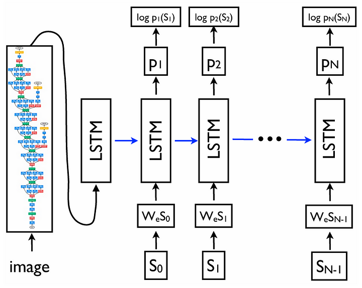
Figure 1. The neural network architecture for image captioning proposed in the Show and Tell paper [2].

Despite having the same encoder-decoder structure, what makes CPTR different from the previous approach is the basis of the encoder and the decoder themselves. In CPTR, we combine the encoder part of the ViT (Vision Transformer) model with the decoder part of the original Transformer model. The use of transformer-based architecture for both components is essentially where the name CPTR comes from: CaPtion TransformeR.

Note that the discussions in this article are going to be highly related to ViT and Transformer, so I highly recommend you read my previous article about these two topics if you’re not yet familiar with them. You can find the links at the end of this article.

Figure 2 shows what the original ViT architecture looks like. Everything inside the green box is the encoder part of the architecture to be adopted as the CPTR encoder.
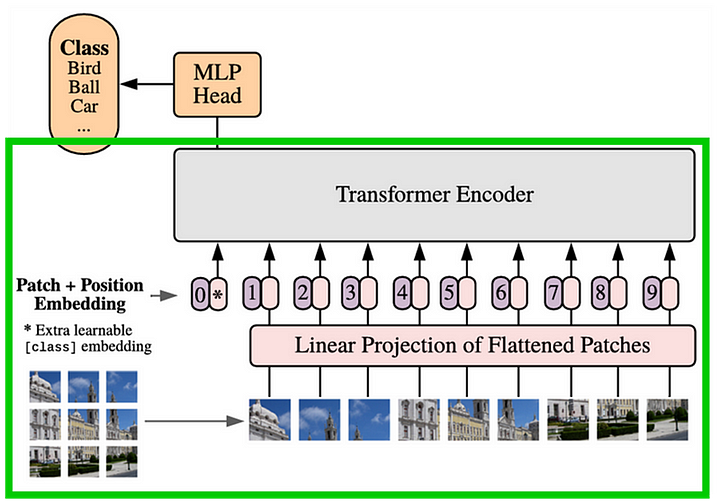
Figure 2. The Vision Transformer (ViT) architecture [3].

Next, Figure 3 displays the original Transformer architecture. The components enclosed in the blue box are the layers that we are going to implement in the CPTR decoder.
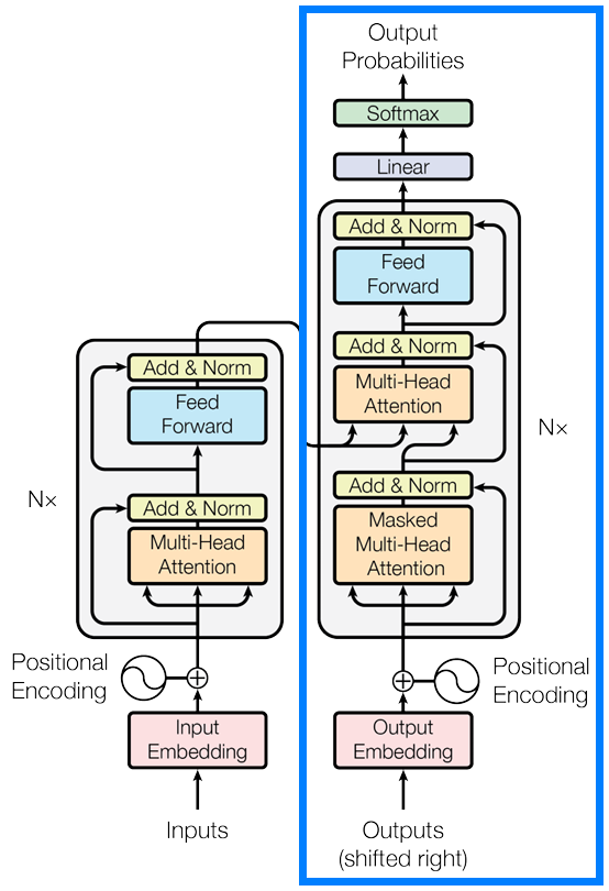
Figure 3. The original Transformer architecture [4].

If we combine the components inside the green and blue boxes above, we are going to obtain the architecture shown in Figure 4 below. This is exactly what the CPTR model we are going to implement looks like. The idea here is that the ViT Encoder (green) works by encoding the input image into a specific tensor representation which will then be used as the basis of the Transformer Decoder (blue) to generate the corresponding caption.
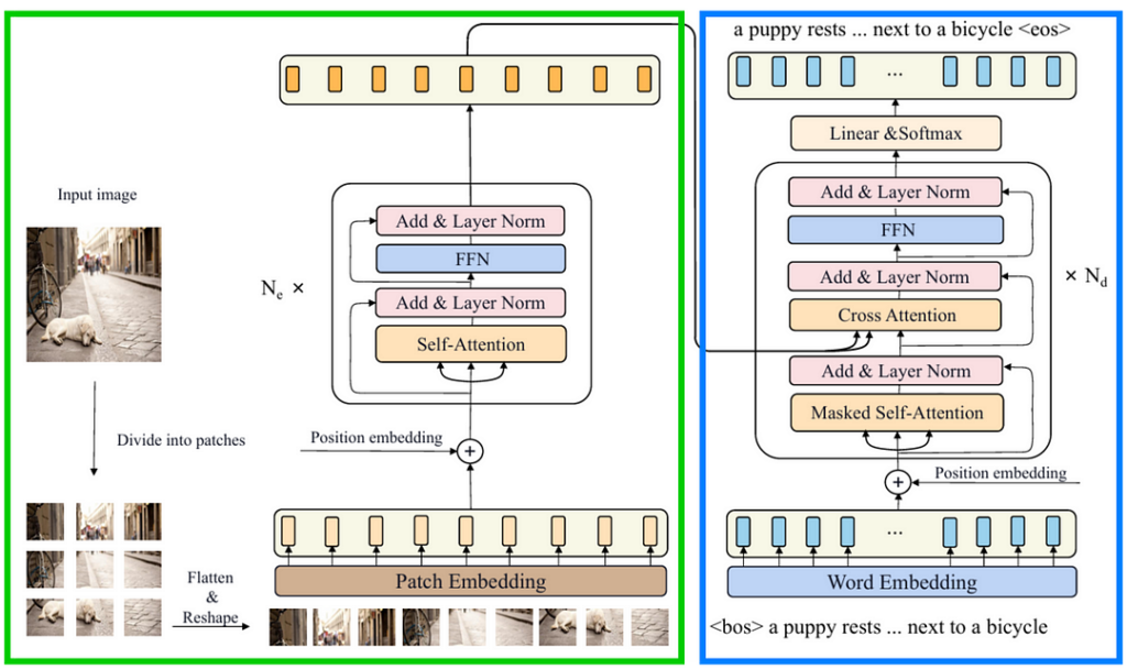
Figure 4. The CPTR architecture [5].

That’s pretty much everything you need to know for now. I’ll explain more about the details as we go through the implementation.

Module imports & parameter configuration

As always, the first thing we need to do in the code is to import the required modules. In this case, we only import torch and torch.nn since we are about to implement the model from scratch.

# Codeblock 1
import torch
import torch.nn as nn

Next, we are going to initialize some parameters in Codeblock 2. If you have read my previous article about image captioning with GoogLeNet and LSTM, you’ll notice that here, we got a lot more parameters to initialize. In this article, I want to reproduce the CPTR model as closely as possible to the original one, so the parameters mentioned in the paper will be used in this implementation.

# Codeblock 2
BATCH_SIZE         = 1              #(1)

IMAGE_SIZE         = 384            #(2)
IN_CHANNELS        = 3              #(3)

SEQ_LENGTH         = 30             #(4)
VOCAB_SIZE         = 10000          #(5)

EMBED_DIM          = 768            #(6)
PATCH_SIZE         = 16             #(7)
NUM_PATCHES        = (IMAGE_SIZE//PATCH_SIZE) ** 2  #(8)
NUM_ENCODER_BLOCKS = 12             #(9)
NUM_DECODER_BLOCKS = 4              #(10)
NUM_HEADS          = 12             #(11)
HIDDEN_DIM         = EMBED_DIM * 4  #(12)
DROP_PROB          = 0.1            #(13)

The first parameter I want to explain is the BATCH_SIZE, which is written at the line marked with #(1). The number assigned to this variable is not quite important in our case since we are not actually going to train this model. This parameter is set to 1 because, by default, PyTorch treats input tensors as a batch of samples. Here I assume that we only have a single sample in a batch. 

Next, remember that in the case of image captioning we are dealing with images and texts simultaneously. This essentially means that we need to set the parameters for the two. It is mentioned in the paper that the model accepts an RGB image of size 384×384 for the encoder input. Hence, we assign the values for IMAGE_SIZE and IN_CHANNELS variables based on this information (#(2) and #(3)). On the other hand, the paper does not mention the parameters for the captions. So, here I assume that the length of the caption is no more than 30 words (#(4)), with the vocabulary size estimated at 10000 unique words (#(5)).

The remaining parameters are related to the model configuration. Here we set the EMBED_DIM variable to 768 (#(6)). In the encoder side, this number indicates the length of the feature vector that represents each 16×16 image patch (#(7)). The same concept also applies to the decoder side, but in that case the feature vector will represent a single word in the caption. Talking more specifically about the PATCH_SIZE parameter, we are going to use the value to compute the total number of patches in the input image. Since the image has the size of 384×384, there will be 576 patches in total (#(8)).

When it comes to using an encoder-decoder architecture, it is possible to specify the number of encoder and decoder blocks to be used. Using more blocks typically allows the model to perform better in terms of the accuracy, yet in return, it will require more computational power. The authors of this paper decided to stack 12 encoder blocks (#(9)) and 4 decoder blocks (#(10)). Next, since CPTR is a transformer-based model, it is necessary to specify the number of attention heads within the attention blocks inside the encoders and the decoders, which in this case authors use 12 attention heads (#(11)). The value for the HIDDEN_DIM parameter is not mentioned anywhere in the paper. However, according to the ViT and the Transformer paper, this parameter is configured to be 4 times larger than EMBED_DIM (#(12)). The dropout rate is not mentioned in the paper either. Hence, I arbitrarily set DROP_PROB to 0.1 (#(13)).

Encoder

As the modules and parameters have been set up, now that we will get into the encoder part of the network. In this section we are going to implement and explain every single component inside the green box in Figure 4 one by one.

Patch embedding
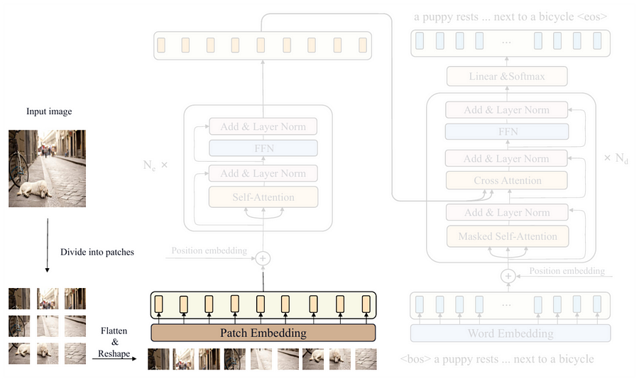
Figure 5. Dividing the input image into patches and converting them into vectors [5].

You can see in Figure 5 above that the first step to be done is dividing the input image into patches. This is essentially done because instead of focusing on local patterns like CNNs, ViT captures global context by learning the relationships between these patches. We can model this process with the Patcher class shown in the Codeblock 3 below. For the sake of simplicity, here I also include the process inside the patch embedding block within the same class.

# Codeblock 3
class Patcher(nn.Module):
   def __init__(self):
       super().__init__()

       #(1)
       self.unfold = nn.Unfold(kernel_size=PATCH_SIZE, stride=PATCH_SIZE)

       #(2)
       self.linear_projection = nn.Linear(in_features=IN_CHANNELS*PATCH_SIZE*PATCH_SIZE,
                                          out_features=EMBED_DIM)
      
   def forward(self, images):
       print(f'imagestt: {images.size()}')
       images = self.unfold(images)  #(3)
       print(f'after unfoldt: {images.size()}')
      
       images = images.permute(0, 2, 1)  #(4)
       print(f'after permutet: {images.size()}')
      
       features = self.linear_projection(images)  #(5)
       print(f'after lin projt: {features.size()}')
      
       return features

The patching itself is done using the nn.Unfold layer (#(1)). Here we need to set both the kernel_size and stride parameters to PATCH_SIZE (16) so that the resulting patches do not overlap with each other. This layer also automatically flattens these patches once it is applied to the input image. Meanwhile, the nn.Linear layer (#(2)) is employed to perform linear projection, i.e., the process done by the patch embedding block. By setting the out_features parameter to EMBED_DIM, this layer will map every single flattened patch into a feature vector of length 768.

The entire process should make more sense once you read the forward() method. You can see at line #(3) in the same codeblock that the input image is directly processed by the unfold layer. Next, we need to process the resulting tensor with the permute() method (#(4)) to swap the first and the second axis before feeding it to the linear_projection layer (#(5)). Additionally, here I also print out the tensor dimension after each layer so that you can better understand the transformation made at each step.

In order to check if our Patcher class works properly, we can just pass a dummy tensor through the network. Look at the Codeblock 4 below to see how I do it.

# Codeblock 4
patcher  = Patcher()

images   = torch.randn(BATCH_SIZE, IN_CHANNELS, IMAGE_SIZE, IMAGE_SIZE)
features = patcher(images)
# Codeblock 4 Output
images         : torch.Size([1, 3, 384, 384])
after unfold   : torch.Size([1, 768, 576])  #(1)
after permute  : torch.Size([1, 576, 768])  #(2)
after lin proj : torch.Size([1, 576, 768])  #(3)

The tensor I passed above represents an RGB image of size 384×384. Here we can see that after the unfold operation is performed, the tensor dimension changed to 1×768×576 (#(1)), denoting the flattened 3×16×16 patch for each of the 576 patches. Unfortunately, this output shape does not match what we need. Remember that in ViT, we perceive image patches as a sequence, so we need to swap the 1st and 2nd axes because typically, the 1st dimension of a tensor represents the temporal axis, while the 2nd one represents the feature vector of each timestep. As the permute() operation is performed, our tensor is now having the dimension of 1×576×768 (#(2)). Lastly, we pass this tensor through the linear projection layer, which the resulting tensor shape remains the same since we set the EMBED_DIM parameter to the same size (768) (#(3)). Despite having the same dimension, the information contained in the final tensor should be richer thanks to the transformation applied by the trainable weights of the linear projection layer.

Learnable positional embedding
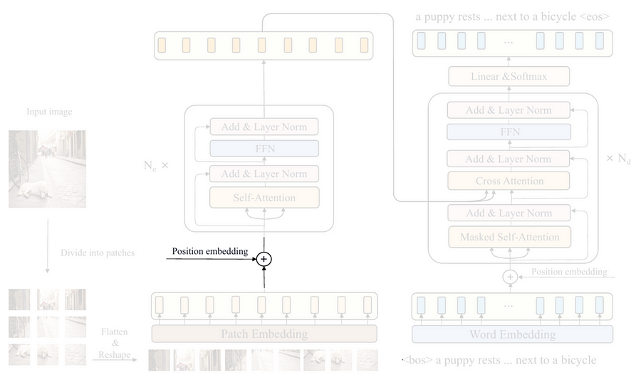
Figure 6. Injecting the learnable positional embeddings into the embedded image patches [5].

After the input image has successfully been converted into a sequence of patches, the next thing to do is to inject the so-called positional embedding tensor. This is essentially done because a transformer without positional embedding is permutation-invariant, meaning that it treats the input sequence as if their order does not matter. Interestingly, since an image is not a literal sequence, we should set the positional embedding to be learnable such that it will be able to somewhat reorder the patch sequence that it thinks works best in representing the spatial information. However, keep in mind that the term “reordering” here does not mean that we physically rearrange the sequence. Rather, it does so by adjusting the embedding weights.

The implementation is pretty simple. All we need to do is just to initialize a tensor using nn.Parameter which the dimension is set to match with the output from the Patcher model, i.e., 576×768. Also, don’t forget to write requires_grad=True just to ensure that the tensor is trainable. Look at the Codeblock 5 below for the details.

# Codeblock 5
class LearnableEmbedding(nn.Module):
   def __init__(self):
       super().__init__()
       self.learnable_embedding = nn.Parameter(torch.randn(size=(NUM_PATCHES, EMBED_DIM)),
                                               requires_grad=True)
      
   def forward(self):
       pos_embed = self.learnable_embedding
       print(f'learnable embeddingt: {pos_embed.size()}')
      
       return pos_embed

Now let’s run the following codeblock to see whether our LearnableEmbedding class works properly. You can see in the printed output that it successfully created the positional embedding tensor as expected.

# Codeblock 6
learnable_embedding = LearnableEmbedding()

pos_embed = learnable_embedding()
# Codeblock 6 Output
learnable embedding : torch.Size([576, 768])

The main encoder block

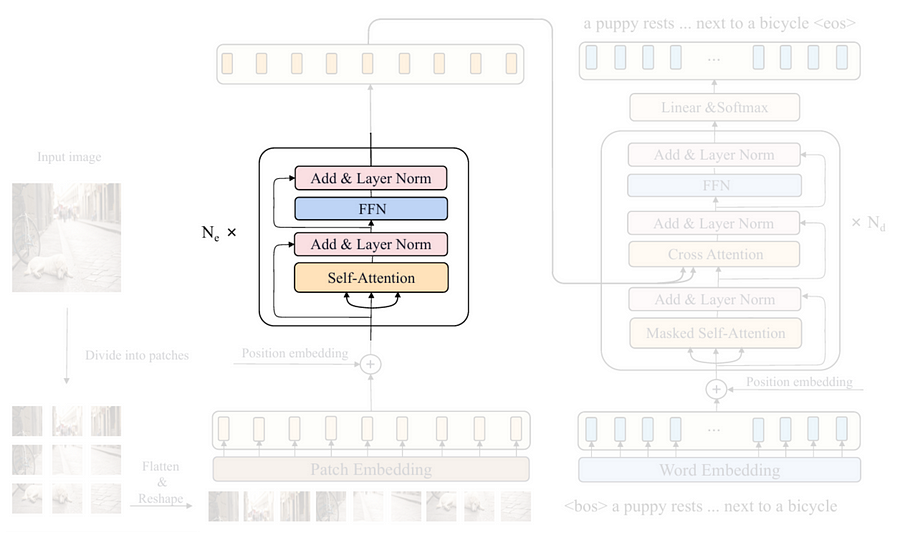
Figure 7. The main encoder block [5].

The next thing we are going to do is to construct the main encoder block displayed in the Figure 7 above. Here you can see that this block consists of several sub-components, namely self-attention, layer norm, FFN (Feed-Forward Network), and another layer norm. The Codeblock 7a below shows how I initialize these layers inside the __init__() method of the EncoderBlock class.

# Codeblock 7a
class EncoderBlock(nn.Module):
   def __init__(self):
       super().__init__()
      
       #(1)
       self.self_attention = nn.MultiheadAttention(embed_dim=EMBED_DIM,
                                                   num_heads=NUM_HEADS,
                                                   batch_first=True,  #(2)
                                                   dropout=DROP_PROB)
      
       self.layer_norm_0 = nn.LayerNorm(EMBED_DIM)  #(3)
      
       self.ffn = nn.Sequential(  #(4)
           nn.Linear(in_features=EMBED_DIM, out_features=HIDDEN_DIM),
           nn.GELU(),
           nn.Dropout(p=DROP_PROB),
           nn.Linear(in_features=HIDDEN_DIM, out_features=EMBED_DIM),
       )
      
       self.layer_norm_1 = nn.LayerNorm(EMBED_DIM)  #(5)

I’ve previously mentioned that the idea of ViT is to capture the relationships between patches within an image. This process is done by the multihead attention layer I initialize at line #(1) in the above codeblock. One thing to keep in mind here is that we need to set the batch_first parameter to True (#(2)). This is essentially done so that the attention layer will be compatible with our tensor shape, in which the batch dimension (batch_size) is at the 0th axis of the tensor. Next, the two layer normalization layers need to be initialized separately, as shown at line #(3) and #(5). Lastly, we initialize the FFN block at line #(4), which the layers stacked using nn.Sequential follows the structure defined in the following equation.

Figure 8. The operations done inside the FFN block [1].

As the __init__() method is complete, we will now continue with the forward() method. Let’s take a look at the Codeblock 7b below.

# Codeblock 7b
   def forward(self, features):  #(1)
      
       residual = features  #(2)
       print(f'features & residualt: {residual.size()}')
      
       #(3)
       features, self_attn_weights = self.self_attention(query=features,
                                                         key=features,
                                                         value=features)
       print(f'after self attentiont: {features.size()}')
       print(f"self attn weightst: {self_attn_weights.shape}")
      
       features = self.layer_norm_0(features + residual)  #(4)
       print(f'after normtt: {features.size()}')
      

       residual = features
       print(f'nfeatures & residualt: {residual.size()}')
      
       features = self.ffn(features)  #(5)
       print(f'after ffntt: {features.size()}')
      
       features = self.layer_norm_1(features + residual)
       print(f'after normtt: {features.size()}')
      
       return features

Here you can see that the input tensor is named features (#(1)). I name it this way because the input of the EncoderBlock is the image that has already been processed with Patcher and LearnableEmbedding, instead of a raw image. Before doing anything, notice in the encoder block that there is a branch separated from the main flow which then returns back to the normalization layer. This branch is commonly known as a residual connection. To implement this, we need to store the original input tensor to the residual variable as I demonstrate at line #(2). As the input tensor has been copied, now we are ready to process the original input with the multihead attention layer (#(3)). Since this is a self-attention (not a cross-attention), the query, key, and value inputs for this layer are all derived from the features tensor. Next, the layer normalization operation is then performed at line #(4), which the input for this layer already contains information from the attention block as well as the residual connection. The remaining steps are basically the same as what I just explained, except that here we replace the self-attention block with FFN (#(5)).

In the following codeblock, I’ll test the EncoderBlock class by passing a dummy tensor of size 1×576×768, simulating an output tensor from the previous operations.

# Codeblock 8
encoder_block = EncoderBlock()

features = torch.randn(BATCH_SIZE, NUM_PATCHES, EMBED_DIM)
features = encoder_block(features)

Below is what the tensor dimension looks like throughout the entire process inside the model.

# Codeblock 8 Output
features & residual  : torch.Size([1, 576, 768])  #(1)
after self attention : torch.Size([1, 576, 768])
self attn weights    : torch.Size([1, 576, 576])  #(2)
after norm           : torch.Size([1, 576, 768])

features & residual  : torch.Size([1, 576, 768])
after ffn            : torch.Size([1, 576, 768])  #(3)
after norm           : torch.Size([1, 576, 768])  #(4)

Here you can see that the final output tensor (#(4)) has the same size as the input (#(1)), allowing us to stack multiple encoder blocks without having to worry about messing up the tensor dimensions. Not only that, the size of the tensor also appears to be unchanged from the beginning all the way to the last layer. In fact, there are actually lots of transformations performed inside the attention block, but we just can’t see it since the entire process is done internally by the nn.MultiheadAttention layer. One of the tensors produced in the layer that we can observe is the attention weight (#(2)). This weight matrix, which has the size of 576×576, is responsible for storing information regarding the relationships between one patch and every other patch in the image. Furthermore, changes in tensor dimension actually also happened inside the FFN layer. The feature vector of each patch which has the initial length of 768 changed to 3072 and immediately shrunk back to 768 again (#(3)). However, this transformation is not printed since the process is wrapped with nn.Sequential back at line #(4) in Codeblock 7a.

ViT encoder

Figure 9. The entire ViT Encoder in the CPTR architecture [5].

As we have finished implementing all encoder components, now that we will assemble them to construct the actual ViT Encoder. We are going to do it in the Encoder class in Codeblock 9.

# Codeblock 9
class Encoder(nn.Module):
   def __init__(self):
       super().__init__()
       self.patcher = Patcher()  #(1)
       self.learnable_embedding = LearnableEmbedding()  #(2)

       #(3)
       self.encoder_blocks = nn.ModuleList(EncoderBlock() for _ in range(NUM_ENCODER_BLOCKS))
  
   def forward(self, images):  #(4)
       print(f'imagesttt: {images.size()}')
      
       features = self.patcher(images)  #(5)
       print(f'after patchertt: {features.size()}')
      
       features = features + self.learnable_embedding()  #(6)
       print(f'after learn embedt: {features.size()}')
      
       for i, encoder_block in enumerate(self.encoder_blocks):
           features = encoder_block(features)  #(7)
           print(f"after encoder block #{i}t: {features.shape}")

       return features

Inside the __init__() method, what we need to do is to initialize all components we created earlier, i.e., Patcher (#(1)), LearnableEmbedding (#(2)), and EncoderBlock (#(3)). In this case, the EncoderBlock is initialized inside nn.ModuleList since we want to repeat it NUM_ENCODER_BLOCKS (12) times. To the forward() method, it initially works by accepting raw image as the input (#(4)). We then process it with the patcher layer (#(5)) to divide the image into small patches and transform them with the linear projection operation. The learnable positional embedding tensor is then injected into the resulting output by element-wise addition (#(6)). Lastly, we pass it into the 12 encoder blocks sequentially with a simple for loop (#(7)).

Now, in Codeblock 10, I am going to pass a dummy image through the entire encoder. Note that since I want to focus on the flow of this Encoder class, I re-run the previous classes we created earlier with the print() functions commented out so that the outputs will look neat.

# Codeblock 10
encoder = Encoder()

images = torch.randn(BATCH_SIZE, IN_CHANNELS, IMAGE_SIZE, IMAGE_SIZE)
features = encoder(images)

And below is what the flow of the tensor looks like. Here, we can see that our dummy input image successfully passed through all layers in the network, including the encoder blocks that we repeat 12 times. The resulting output tensor is now context-aware, meaning that it already contains information about the relationships between patches within the image. Therefore, this tensor is now ready to be processed further with the decoder, which will later be discussed in the subsequent section.

# Codeblock 10 Output
images                  : torch.Size([1, 3, 384, 384])
after patcher           : torch.Size([1, 576, 768])
after learn embed       : torch.Size([1, 576, 768])
after encoder block #0  : torch.Size([1, 576, 768])
after encoder block #1  : torch.Size([1, 576, 768])
after encoder block #2  : torch.Size([1, 576, 768])
after encoder block #3  : torch.Size([1, 576, 768])
after encoder block #4  : torch.Size([1, 576, 768])
after encoder block #5  : torch.Size([1, 576, 768])
after encoder block #6  : torch.Size([1, 576, 768])
after encoder block #7  : torch.Size([1, 576, 768])
after encoder block #8  : torch.Size([1, 576, 768])
after encoder block #9  : torch.Size([1, 576, 768])
after encoder block #10 : torch.Size([1, 576, 768])
after encoder block #11 : torch.Size([1, 576, 768])

ViT encoder (alternative)

I want to show you something before we talk about the decoder. If you think that our approach above is too complicated, it is actually possible for you to use nn.TransformerEncoderLayer from PyTorch so that you don’t need to implement the EncoderBlock class from scratch. To do so, I am going to reimplement the Encoder class, but this time I’ll name it EncoderTorch.

# Codeblock 11
class EncoderTorch(nn.Module):
   def __init__(self):
       super().__init__()
       self.patcher = Patcher()
       self.learnable_embedding = LearnableEmbedding()
      
       #(1)
       encoder_block = nn.TransformerEncoderLayer(d_model=EMBED_DIM,
                                                  nhead=NUM_HEADS,
                                                  dim_feedforward=HIDDEN_DIM,
                                                  dropout=DROP_PROB,
                                                  batch_first=True)
      
       #(2)
       self.encoder_blocks = nn.TransformerEncoder(encoder_layer=encoder_block,
                                                   num_layers=NUM_ENCODER_BLOCKS)
  
   def forward(self, images):
       print(f'imagesttt: {images.size()}')
      
       features = self.patcher(images)
       print(f'after patchertt: {features.size()}')
      
       features = features + self.learnable_embedding()
       print(f'after learn embedt: {features.size()}')
      
       features = self.encoder_blocks(features)  #(3)
       print(f'after encoder blockst: {features.size()}')

       return features

What we basically do in the above codeblock is that instead of using the EncoderBlock class, here we use nn.TransformerEncoderLayer (#(1)), which will automatically create a single encoder block based on the parameters we pass to it. To repeat it multiple times, we can just use nn.TransformerEncoder and pass a number to the num_layers parameter (#(2)). With this approach, we don’t necessarily need to write the forward pass in a loop like what we did earlier (#(3)).

The testing code in the Codeblock 12 below is exactly the same as the one in Codeblock 10, except that here I use the EncoderTorch class. You can also see here that the output is basically the same as the previous one.

# Codeblock 12
encoder_torch = EncoderTorch()

images = torch.randn(BATCH_SIZE, IN_CHANNELS, IMAGE_SIZE, IMAGE_SIZE)
features = encoder_torch(images)
# Codeblock 12 Output
images               : torch.Size([1, 3, 384, 384])
after patcher        : torch.Size([1, 576, 768])
after learn embed    : torch.Size([1, 576, 768])
after encoder blocks : torch.Size([1, 576, 768])

Decoder

As we have successfully created the encoder part of the CPTR architecture, now that we will talk about the decoder. In this section I am going to implement every single component inside the blue box in Figure 4. Based on the figure, we can see that the decoder accepts two inputs, i.e., the image caption ground truth (the lower part of the blue box) and the sequence of embedded patches produced by the encoder (the arrow coming from the green box). It is important to know that the architecture drawn in Figure 4 is intended to illustrate the training phase, where the entire caption ground truth is fed into the decoder. Later in the inference phase, we only provide a (Beginning of Sentence) token for the caption input. The decoder will then predict each word sequentially based on the given image and the previously generated words. This process is commonly known as an autoregressive mechanism.

Sinusoidal positional embedding
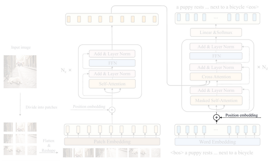
Figure 10. Where the sinusoidal positional embedding component is located in the decoder [5].

If you take a look at the CPTR model, you’ll see that the first step in the decoder is to convert each word into the corresponding feature vector representation using the word embedding block. However, since this step is very easy, we are going to implement it later. Now let’s assume that this word vectorization process is already done, so we can move to the positional embedding part.

As I’ve mentioned earlier, since transformer is permutation-invariant by nature, we need to apply positional embedding to the input sequence. Different from the previous one, here we use the so-called sinusoidal positional embedding. We can think of it like a method to label each word vector by assigning numbers obtained from a sinusoidal wave. By doing so, we can expect our model to understand word orders thanks to the information given by the wave patterns.

If you go back to Codeblock 6 Output, you’ll see that the positional embedding tensor in the encoder has the size of NUM_PATCHES × EMBED_DIM (576×768). What we basically want to do in the decoder is to create a tensor having the size of SEQ_LENGTH × EMBED_DIM (30×768), which the values are computed based on the equation shown in Figure 11. This tensor is then set to be non-trainable because a sequence of words must maintain a fixed order to preserve its meaning.

Figure 11. The equation for creating sinusoidal positional encoding proposed in the Transformer paper [6].

Here I want to explain the following code quickly because I actually have discussed this more thoroughly in my previous article about Transformer. Generally speaking, what we basically do here is to create the sine and cosine wave using torch.sin() (#(1)) and torch.cos() (#(2)). The resulting two tensors are then merged using the code at line #(3) and #(4).

# Codeblock 13
class SinusoidalEmbedding(nn.Module):
   def forward(self):
       pos = torch.arange(SEQ_LENGTH).reshape(SEQ_LENGTH, 1)
       print(f"postt: {pos.shape}")
      
       i = torch.arange(0, EMBED_DIM, 2)
       denominator = torch.pow(10000, i/EMBED_DIM)
       print(f"denominatort: {denominator.shape}")
      
       even_pos_embed = torch.sin(pos/denominator)  #(1)
       odd_pos_embed  = torch.cos(pos/denominator)  #(2)
       print(f"even_pos_embedt: {even_pos_embed.shape}")
      
       stacked = torch.stack([even_pos_embed, odd_pos_embed], dim=2)  #(3)
       print(f"stackedtt: {stacked.shape}")

       pos_embed = torch.flatten(stacked, start_dim=1, end_dim=2)  #(4)
       print(f"pos_embedt: {pos_embed.shape}")
      
       return pos_embed

Now we can check if the SinusoidalEmbedding class above works properly by running the Codeblock 14 below. As expected earlier, here you can see that the resulting tensor has the size of 30×768. This dimension matches with the tensor obtained by the process done in the word embedding block, allowing them to be summed in an element-wise manner.

# Codeblock 14
sinusoidal_embedding = SinusoidalEmbedding()
pos_embed = sinusoidal_embedding()
# Codeblock 14 Output
pos            : torch.Size([30, 1])
denominator    : torch.Size([384])
even_pos_embed : torch.Size([30, 384])
stacked        : torch.Size([30, 384, 2])
pos_embed      : torch.Size([30, 768])

Look-ahead mask

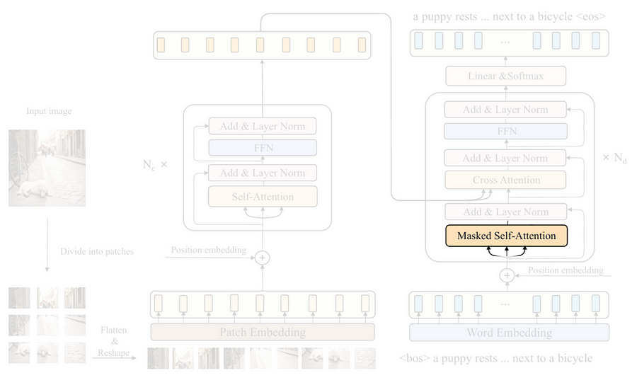
Figure 12. A look-ahead mask needs to be applied to the masked-self attention layer [5].

The next thing I am going to talk about in the decoder is the masked self-attention layer highlighted in the above figure. I am not going to code the attention mechanism from scratch. Rather, I’ll only implement the so-called look-ahead mask, which will be useful for the self-attention layer so that it doesn’t attend to the subsequent words in the caption during the training phase.

The way to do it is pretty easy, what we need to do is just to create a triangular matrix which the size is set to match with the attention weight matrix, i.e., SEQ_LENGTH × SEQ_LENGTH (30×30). Look at the create_mask()function below for the details.

# Codeblock 15
def create_mask(seq_length):
   mask = torch.tril(torch.ones((seq_length, seq_length)))  #(1)
   mask[mask == 0] = -float('inf')  #(2)
   mask[mask == 1] = 0  #(3)
   return mask

Even though creating a triangular matrix can simply be done with torch.tril() and torch.ones() (#(1)), but here we need to make a little modification by changing the 0 values to -inf (#(2)) and the 1s to 0 (#(3)). This is essentially done because the nn.MultiheadAttention layer applies the mask by element-wise addition. By assigning -inf to the subsequent words, the attention mechanism will completely ignore them. Again, the internal process inside an attention layer has also been discussed in detail in my previous article about transformer.

Now I am going to run the function with seq_length=7 so that you can see what the mask actually looks like. Later in the complete flow, we need to set the seq_length parameter to SEQ_LENGTH (30) so that it matches with the actual caption length.

# Codeblock 16
mask_example = create_mask(seq_length=7)
mask_example
# Codeblock 16 Output
tensor([[0., -inf, -inf, -inf, -inf, -inf, -inf],
       [0., 0., -inf, -inf, -inf, -inf, -inf],
       [0., 0., 0., -inf, -inf, -inf, -inf],
       [0., 0., 0., 0., -inf, -inf, -inf],
       [0., 0., 0., 0., 0., -inf, -inf],
       [0., 0., 0., 0., 0., 0., -inf],
       [0., 0., 0., 0., 0., 0., 0.]])

The main decoder block

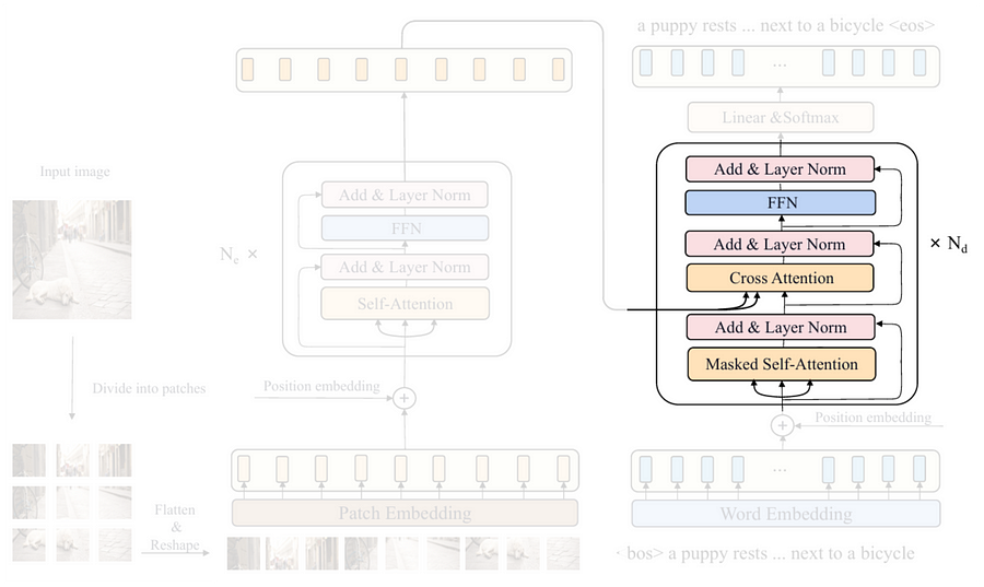
Figure 13. The main decoder block [5].

We can see in the above figure that the structure of the decoder block is a bit longer than that of the encoder block. It seems like everything is nearly the same, except that the decoder part has a cross-attention mechanism and an additional layer normalization step placed after it. This cross-attention layer can actually be perceived as the bridge between the encoder and the decoder, as it is employed to capture the relationships between each word in the caption and every single patch in the input image. The two arrows coming from the encoder are the key and value inputs for the attention layer, whereas the query is derived from the previous layer in the decoder itself. Look at the Codeblock 17a and 17b below to see the implementation of the entire decoder block.

# Codeblock 17a
class DecoderBlock(nn.Module):
   def __init__(self):
       super().__init__()
      
       #(1)
       self.self_attention = nn.MultiheadAttention(embed_dim=EMBED_DIM,
                                                   num_heads=NUM_HEADS,
                                                   batch_first=True,
                                                   dropout=DROP_PROB)
       #(2)
       self.layer_norm_0 = nn.LayerNorm(EMBED_DIM)
       #(3)
       self.cross_attention = nn.MultiheadAttention(embed_dim=EMBED_DIM,
                                                    num_heads=NUM_HEADS,
                                                    batch_first=True,
                                                    dropout=DROP_PROB)

       #(4)
       self.layer_norm_1 = nn.LayerNorm(EMBED_DIM)
      
       #(5)      
       self.ffn = nn.Sequential(
           nn.Linear(in_features=EMBED_DIM, out_features=HIDDEN_DIM),
           nn.GELU(),
           nn.Dropout(p=DROP_PROB),
           nn.Linear(in_features=HIDDEN_DIM, out_features=EMBED_DIM),
       )
      
       #(6)
       self.layer_norm_2 = nn.LayerNorm(EMBED_DIM)

In the __init__() method, we first initialize both self-attention (#(1)) and cross-attention (#(3)) layers with nn.MultiheadAttention. These two layers appear to be exactly the same now, but later you’ll see the difference in the forward() method. The three layer normalization operations are initialized separately as shown at line #(2), #(4) and #(6), since each of them will contain different normalization parameters. Lastly, the ffn layer (#(5)) is exactly the same as the one in the encoder, which basically follows the equation back in Figure 8.

Talking about the forward() method below, it initially works by accepting three inputs: features, captions, and attn_mask, which each of them denotes the tensor coming from the encoder, the tensor from the decoder itself, and a look-ahead mask, respectively (#(1)). The remaining steps are somewhat similar to that of the EncoderBlock, except that here we repeat the multihead attention block twice. The first attention mechanism takes captions as the query, key, and value parameters (#(2)). This is essentially done because we want the layer to capture the context within the captions tensor itself — hence the name self-attention. Here we also need to pass the attn_mask parameter to this layer so that it cannot see the subsequent words during the training phase. The second attention mechanism is different (#(3)). Since we want to combine the information from the encoder and the decoder, we need to pass the captions tensor as the query, whereas the features tensor will be passed as the key and value — hence the name cross-attention. A look-ahead mask is not necessary in the cross-attention layer since later in the inference phase the model will be able to see the entire input image at once rather than looking at the patches one by one. As the tensor has been processed by the two attention layers, we will then pass it through the feed forward network (#(4)). Lastly, don’t forget to create the residual connections and apply the layer normalization steps after each sub-component.

# Codeblock 17b
   def forward(self, features, captions, attn_mask):  #(1)
       print(f"attn_masktt: {attn_mask.shape}")
       residual = captions
       print(f"captions & residualt: {captions.shape}")
      
       #(2)
       captions, self_attn_weights = self.self_attention(query=captions,
                                                         key=captions,
                                                         value=captions,
                                                         attn_mask=attn_mask)
       print(f"after self attentiont: {captions.shape}")
       print(f"self attn weightst: {self_attn_weights.shape}")
      
       captions = self.layer_norm_0(captions + residual)
       print(f"after normtt: {captions.shape}")
      
      
       print(f"nfeaturestt: {features.shape}")
       residual = captions
       print(f"captions & residualt: {captions.shape}")
      
       #(3)
       captions, cross_attn_weights = self.cross_attention(query=captions,
                                                           key=features,
                                                           value=features)
       print(f"after cross attentiont: {captions.shape}")
       print(f"cross attn weightst: {cross_attn_weights.shape}")
      
       captions = self.layer_norm_1(captions + residual)
       print(f"after normtt: {captions.shape}")
      
       residual = captions
       print(f"ncaptions & residualt: {captions.shape}")
      
       captions = self.ffn(captions)  #(4)
       print(f"after ffntt: {captions.shape}")
      
       captions = self.layer_norm_2(captions + residual)
       print(f"after normtt: {captions.shape}")
      
       return captions

As the DecoderBlock class is completed, we can now test it with the following code.

# Codeblock 18
decoder_block = DecoderBlock()

features = torch.randn(BATCH_SIZE, NUM_PATCHES, EMBED_DIM)  #(1)
captions = torch.randn(BATCH_SIZE, SEQ_LENGTH, EMBED_DIM)   #(2)
look_ahead_mask = create_mask(seq_length=SEQ_LENGTH)  #(3)

captions = decoder_block(features, captions, look_ahead_mask)

Here we assume that features is a tensor containing a sequence of patch embeddings produced by the encoder (#(1)), while captions is a sequence of embedded words (#(2)). The seq_length parameter of the look-ahead mask is set to SEQ_LENGTH (30) to match it to the number of words in the caption (#(3)). The tensor dimensions after each step are displayed in the following output.

# Codeblock 18 Output
attn_mask             : torch.Size([30, 30])
captions & residual   : torch.Size([1, 30, 768])
after self attention  : torch.Size([1, 30, 768])
self attn weights     : torch.Size([1, 30, 30])    #(1)
after norm            : torch.Size([1, 30, 768])

features              : torch.Size([1, 576, 768])
captions & residual   : torch.Size([1, 30, 768])
after cross attention : torch.Size([1, 30, 768])
cross attn weights    : torch.Size([1, 30, 576])   #(2)
after norm            : torch.Size([1, 30, 768])

captions & residual   : torch.Size([1, 30, 768])
after ffn             : torch.Size([1, 30, 768])
after norm            : torch.Size([1, 30, 768])

Here we can see that our DecoderBlock class works properly as it successfully processed the input tensors all the way to the last layer in the network. Here I want you to take a closer look at the attention weights at lines #(1) and #(2). Based on these two lines, we can confirm that our decoder implementation is correct since the attention weight produced by the self-attention layer has the size of 30×30 (#(1)), which basically means that this layer really captured the context within the input caption. Meanwhile, the attention weight matrix generated by the cross-attention layer has the size of 30×576 (#(2)), indicating that it successfully captured the relationships between the words and the patches. This essentially implies that after cross-attention operation is performed, the resulting captions tensor has been enriched with the information from the image.

Transformer decoder
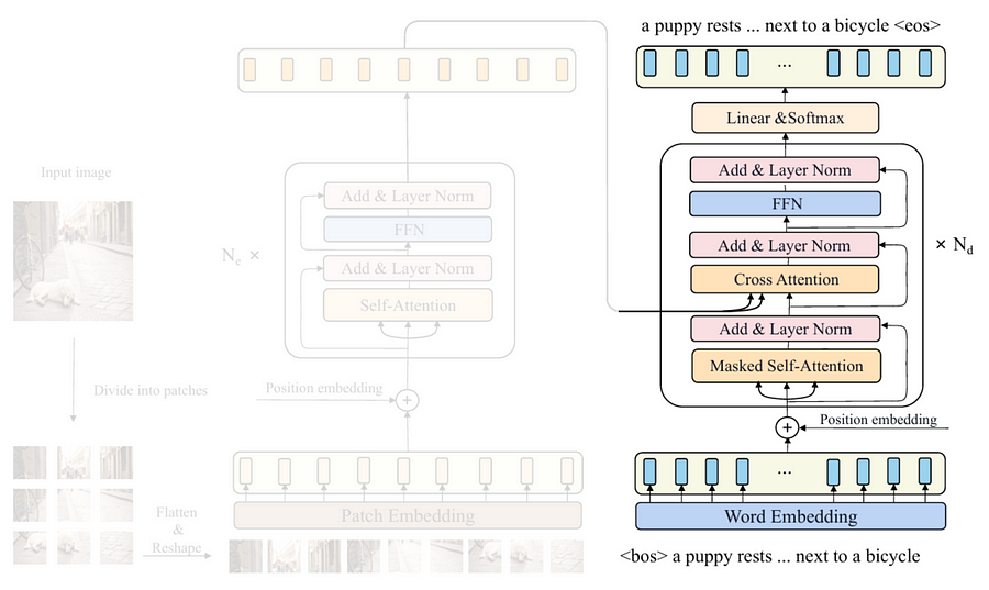
Figure 14. The entire Transformer Decoder in the CPTR architecture [5].

Now that we have successfully created all components for the entire decoder, what I am going to do next is to put them together into a single class. Look at the Codeblock 19a and 19b below to see how I do that.

# Codeblock 19a
class Decoder(nn.Module):
   def __init__(self):
       super().__init__()

       #(1)
       self.embedding = nn.Embedding(num_embeddings=VOCAB_SIZE,
                                     embedding_dim=EMBED_DIM)

       #(2)
       self.sinusoidal_embedding = SinusoidalEmbedding()

       #(3)
       self.decoder_blocks = nn.ModuleList(DecoderBlock() for _ in range(NUM_DECODER_BLOCKS))

       #(4)
       self.linear = nn.Linear(in_features=EMBED_DIM,
                               out_features=VOCAB_SIZE)

If you compare this Decoder class with the Encoder class from codeblock 9, you’ll notice that they are somewhat similar in terms of the structure. In the encoder, we convert image patches into vectors using Patcher, while in the decoder we convert every single word in the caption into a vector using the nn.Embedding layer (#(1)), which I haven’t explained earlier. Afterward, we initialize the positional embedding layer, where for the decoder we use the sinusoidal rather than the trainable one (#(2)). Next, we stack multiple decoder blocks using nn.ModuleList (#(3)). The linear layer written at line #(4), which doesn’t exist in the encoder, is necessary to be implemented here since it will be responsible to map each of the embedded words into a vector of length VOCAB_SIZE (10000). Later on, this vector will contain the logit of every word in the dictionary, and what we need to do afterward is just to take the index containing the highest value, i.e., the most likely word to be predicted.

The flow of the tensors within the forward() method itself is also pretty similar to the one in the Encoder class. In the Codeblock 19b below we pass features, captions, and attn_mask as the input (#(1)). Keep in mind that in this case the captions tensor contains the raw word sequence, so we need to vectorize these words with the embedding layer beforehand (#(2)). Next, we inject the sinusoidal positional embedding tensor using the code at line #(3) before eventually passing it through the four decoder blocks sequentially (#(4)). Finally, we pass the resulting tensor through the last linear layer to obtain the prediction logits (#(5)).

# Codeblock 19b
   def forward(self, features, captions, attn_mask):  #(1)
       print(f"featurestt: {features.shape}")
       print(f"captionstt: {captions.shape}")
      
       captions = self.embedding(captions)  #(2)
       print(f"after embeddingtt: {captions.shape}")
      
       captions = captions + self.sinusoidal_embedding()  #(3)
       print(f"after sin embedtt: {captions.shape}")
      
       for i, decoder_block in enumerate(self.decoder_blocks):
           captions = decoder_block(features, captions, attn_mask)  #(4)
           print(f"after decoder block #{i}t: {captions.shape}")
      
       captions = self.linear(captions)  #(5)
       print(f"after lineartt: {captions.shape}")
      
       return captions

At this point you might be wondering why we don’t implement the softmax activation function as drawn in the illustration. This is essentially because during the training phase, softmax is typically included within the loss function, whereas in the inference phase, the index of the largest value will remain the same regardless of whether softmax is applied.

Now let’s run the following testing code to check whether there are errors in our implementation. Previously I mentioned that the captions input of the Decoder class is a raw word sequence. To simulate this, we can simply create a sequence of random integers ranging between 0 and VOCAB_SIZE (10000) with the length of SEQ_LENGTH (30) words (#(1)).

# Codeblock 20
decoder = Decoder()

features = torch.randn(BATCH_SIZE, NUM_PATCHES, EMBED_DIM)
captions = torch.randint(0, VOCAB_SIZE, (BATCH_SIZE, SEQ_LENGTH))  #(1)

captions = decoder(features, captions, look_ahead_mask)

And below is what the resulting output looks like. Here you can see in the last line that the linear layer produced a tensor of size 30×10000, indicating that our decoder model is now capable of predicting the logit scores for each word in the vocabulary across all 30 sequence positions.

# Codeblock 20 Output
features               : torch.Size([1, 576, 768])
captions               : torch.Size([1, 30])
after embedding        : torch.Size([1, 30, 768])
after sin embed        : torch.Size([1, 30, 768])
after decoder block #0 : torch.Size([1, 30, 768])
after decoder block #1 : torch.Size([1, 30, 768])
after decoder block #2 : torch.Size([1, 30, 768])
after decoder block #3 : torch.Size([1, 30, 768])
after linear           : torch.Size([1, 30, 10000])

Transformer decoder (alternative)

It is actually also possible to make the code simpler by replacing the DecoderBlock class with the nn.TransformerDecoderLayer, just like what we did in the ViT Encoder. Below is what the code looks like if we use this approach instead.

# Codeblock 21
class DecoderTorch(nn.Module):
   def __init__(self):
       super().__init__()
       self.embedding = nn.Embedding(num_embeddings=VOCAB_SIZE,
                                     embedding_dim=EMBED_DIM)
      
       self.sinusoidal_embedding = SinusoidalEmbedding()
      
       #(1)
       decoder_block = nn.TransformerDecoderLayer(d_model=EMBED_DIM,
                                                  nhead=NUM_HEADS,
                                                  dim_feedforward=HIDDEN_DIM,
                                                  dropout=DROP_PROB,
                                                  batch_first=True)
      
       #(2)
       self.decoder_blocks = nn.TransformerDecoder(decoder_layer=decoder_block,
                                                   num_layers=NUM_DECODER_BLOCKS)
      
       self.linear = nn.Linear(in_features=EMBED_DIM,
                               out_features=VOCAB_SIZE)
      
   def forward(self, features, captions, tgt_mask):
       print(f"featurestt: {features.shape}")
       print(f"captionstt: {captions.shape}")
      
       captions = self.embedding(captions)
       print(f"after embeddingtt: {captions.shape}")
      
       captions = captions + self.sinusoidal_embedding()
       print(f"after sin embedtt: {captions.shape}")
      
       #(3)
       captions = self.decoder_blocks(tgt=captions,
                                      memory=features,
                                      tgt_mask=tgt_mask)
       print(f"after decoder blockst: {captions.shape}")
      
       captions = self.linear(captions)
       print(f"after lineartt: {captions.shape}")
      
       return captions

The main difference you will see in the __init__() method is the use of nn.TransformerDecoderLayer and nn.TransformerDecoder at line #(1) and #(2), where the former is used to initialize a single decoder block, and the latter is for repeating the block multiple times. Next, the forward() method is mostly similar to the one in the Decoder class, except that the forward propagation on the decoder blocks is automatically repeated four times without needing to be put inside a loop (#(3)). One thing that you need to pay attention to in the decoder_blocks layer is that the tensor coming from the encoder (features) must be passed as the argument for the memory parameter. Meanwhile, the tensor from the decoder itself (captions) has to be passed as the input to the tgt parameter.

The testing code for the DecoderTorch model below is basically the same as the one written in Codeblock 20. Here you can see that this model also generates the final output tensor of size 30×10000.

# Codeblock 22
decoder_torch = DecoderTorch()

features = torch.randn(BATCH_SIZE, NUM_PATCHES, EMBED_DIM)
captions = torch.randint(0, VOCAB_SIZE, (BATCH_SIZE, SEQ_LENGTH))

captions = decoder_torch(features, captions, look_ahead_mask)
# Codeblock 22 Output
features             : torch.Size([1, 576, 768])
captions             : torch.Size([1, 30])
after embedding      : torch.Size([1, 30, 768])
after sin embed      : torch.Size([1, 30, 768])
after decoder blocks : torch.Size([1, 30, 768])
after linear         : torch.Size([1, 30, 10000])

The entire CPTR model

Finally, it’s time to put the encoder and the decoder part we just created into a single class to actually construct the CPTR architecture. You can see in Codeblock 23 below that the implementation is very simple. All we need to do here is just to initialize the encoder (#(1)) and the decoder (#(2)) components, then pass the raw images and the corresponding caption ground truths as well as the look-ahead mask to the forward() method (#(3)). Additionally, it is also possible for you to replace the Encoder and the Decoder with EncoderTorch and DecoderTorch, respectively.

# Codeblock 23
class EncoderDecoder(nn.Module):
   def __init__(self):
       super().__init__()
       self.encoder = Encoder()  #EncoderTorch()  #(1)
       self.decoder = Decoder()  #DecoderTorch()  #(2)
      
   def forward(self, images, captions, look_ahead_mask):  #(3)
       print(f"imagesttt: {images.shape}")
       print(f"captionstt: {captions.shape}")
      
       features = self.encoder(images)
       print(f"after encodertt: {features.shape}")
      
       captions = self.decoder(features, captions, look_ahead_mask)
       print(f"after decodertt: {captions.shape}")
      
       return captions

We can do the testing by passing dummy tensors through it. See the Codeblock 24 below for the details. In this case, images is basically just a tensor of random numbers having the dimension of 1×3×384×384 (#(1)), while captions is a tensor of size 1×30 containing random integers (#(2)).

# Codeblock 24
encoder_decoder = EncoderDecoder()

images = torch.randn(BATCH_SIZE, IN_CHANNELS, IMAGE_SIZE, IMAGE_SIZE)  #(1)
captions = torch.randint(0, VOCAB_SIZE, (BATCH_SIZE, SEQ_LENGTH))  #(2)

captions = encoder_decoder(images, captions, look_ahead_mask)

Below is what the output looks like. We can see here that our input images and captions successfully went through all layers in the network, which basically means that the CPTR model we created is now ready to actually be trained on image captioning datasets.

# Codeblock 24 Output
images         : torch.Size([1, 3, 384, 384])
captions       : torch.Size([1, 30])
after encoder  : torch.Size([1, 576, 768])
after decoder  : torch.Size([1, 30, 10000])

Ending

That was pretty much everything about the theory and implementation of the CaPtion TransformeR architecture. Let me know what deep learning architecture I should implement next. Feel free to leave a comment if you spot any mistakes in this article!

The code used in this article is available in my GitHub repo. Here’s the link to my previous article about image captioning, Vision Transformer (ViT), and the original Transformer.

References

[1] Wei Liu et al. CPTR: Full Transformer Network for Image Captioning. Arxiv. https://arxiv.org/pdf/2101.10804 [Accessed November 16, 2024].

[2] Oriol Vinyals et al. Show and Tell: A Neural Image Caption Generator. Arxiv. https://arxiv.org/pdf/1411.4555 [Accessed December 3, 2024].

[3] Image originally created by author based on: Alexey Dosovitskiy et al. An Image is Worth 16×16 Words: Transformers for Image Recognition at Scale. Arxiv. https://arxiv.org/pdf/2010.11929 [Accessed December 3, 2024].

[4] Image originally created by author based on [6].

[5] Image originally created by author based on [1].

[6] Ashish Vaswani et al. Attention Is All You Need. Arxiv. https://arxiv.org/pdf/1706.03762 [Accessed December 3, 2024].


Shape
Shape
Stay Ahead

Explore More Insights

Stay ahead with more perspectives on cutting-edge power, infrastructure, energy,  bitcoin and AI solutions. Explore these articles to uncover strategies and insights shaping the future of industries.

Shape

Why 6 GHz Wi-Fi will make or break the modern enterprise

To date, 6 GHz Wi‑Fi deployments across enterprises remain in their early stages, with only a subset of organizations moving aggressively beyond Wi‑Fi 6 and legacy bands. Most corporate campuses, manufacturing plants, healthcare facilities, and retail environments continue to run primarily on 2.4 GHz and 5 GHz, even as their

Read More »

IBM partners with OpenAI to drive enterprise AI deployment

There will be three focus areas in the new partnership: helping organizations transform their businesses to integrate AI into their daily work, assisting clients in modernizing legacy applications through a combination of OpenAI products and IBM’s expertise, and an expansion of an existing cybersecurity collaboration combining OpenAI frontier AI capabilities

Read More »

Cisco rides ‘networking supercycle’ for strong Q4

Security revenue grew 14% year-over-year in Q4, with more than 1,500 customers adopting new products such as Secure Access, XDR, HyperShield, and AI Defense, bringing the total new customer count for these products to 6,400 since launch, Robbins noted. Firewall orders increased more than 30%, and AI security features like AI

Read More »

Equinor lets stimulation service contract for NCS assets

@import url(‘https://fonts.googleapis.com/css2?family=Inter:wght@100..900&display=swap’); .ebm-page__main h1, .ebm-page__main h2, .ebm-page__main h3, .ebm-page__main h4, .ebm-page__main h5, .ebm-page__main h6 { font-family: Inter; } body { line-height: 150%; letter-spacing: 0.025em; } button, .ebm-button-wrapper { font-family: Inter; } .label-style { text-transform: uppercase; color: var(–color-grey); font-weight: 600; font-size: 0.75rem; } .caption-style { font-size: 0.75rem; opacity: .6; } #onetrust-pc-sdk

Read More »

Energy Secretary Keeps Coal-Fired Generation Operational in the Midwest

WASHINGTON—U.S. Secretary of Energy Chris Wright issued an emergency order to address critical grid reliability issues in the Midwest. The emergency order directs the Midwest Independent System Operator (MISO), in coordination with Consumers Energy, to ensure that the 1,420-megawatt (MW) J.H. Campbell coal-fired power plant (Campbell Plant) in West Olive, Michigan is available to operate and to employ economic dispatch to minimize costs for American families and businesses. The Campbell Plant was originally scheduled to shut down on May 31, 2025, 15 years before the end of its scheduled design life. Since the U.S. Department of Energy’s (DOE) original order issued on May 23, 2205, the Campbell Plant has proven critical to MISO’s operations, operating regularly during periods of high energy demand and low levels of intermittent energy production. Subsequent orders were issued throughout 2025 and 2026. This order is in effect beginning on August 17, 2026, through November 14, 2026. “President Trump and the Energy Department remain committed to doing everything in our power to mitigate the possibility of power outages for American families and businesses,” Secretary Wright said. “Ensuring coal plants such as the Campbell Plant are available to operate during periods of high electricity demand saves lives. Americans deserve access to affordable, reliable, and secure electricity regardless of whether the wind is blowing or the sun is shining.” In January 2026, North American Electric Reliability Corporation (NERC) released its 2025 Long-Term Reliability Assessment. NERC assessed that the MISO region is at high risk of energy shortfalls over the next five years, stating that it faces significant reliability challenges as “projected resource additions do not keep pace with escalating demand forecasts and announced generator retirements.” NERC released its 2026 State of Reliability (SOR) on June 4, 2026. In its technical discussion of major system events, NERC states “shoulder reasons

Read More »

Hydrocarbons and Geothermal Energy Office Announces Up to $10.75 Million to Support University Training and Research for Subsurface Energy Development

WASHINGTON—The U.S. Department of Energy’s (DOE) Hydrocarbons and Geothermal Energy Office (HGEO) today announced up to $10.75 million in federal funding to support novel, early-stage research and development (R&D) projects at eligible U.S. colleges and universities. The funding opportunity is offered through HGEO’s University Training and Research (UTR) Program, which aims to train the next generation of engineers and scientists for careers in energy-related research to help ensure affordable, reliable, and secure energy for all Americans. “Continuing to increase domestic energy production from our vast coal, oil, gas, and geothermal resources requires a workforce of trained, qualified professionals to advance innovative subsurface energy technologies,” said DOE Acting Assistant Secretary of the Hydrocarbons and Geothermal Energy Office Curt Coccodrilli. “By investing in skills-based training that emphasizes industry-driven strategies, we will help meet the needs of our evolving energy economy while strengthening America’s energy leadership and independence.”  Funding awarded under this notice of funding opportunity (NOFO) is intended to increase R&D opportunities for students in science, technology, engineering and mathematics. Relevant academic disciplines include, but are not limited to engineering, chemistry, physics, mining, geosciences, computer science and education.  Selected projects will support one topic area—Innovative Research and Training for Subsurface Energy Production. This topic area seeks university-led R&D proposals focused on accelerating innovative energy technologies toward commercial viability while simultaneously developing a skilled workforce for the evolving energy sector. The topic area is split into three subtopics  focused on coal, oil and gas, and geothermal energy, respectively, ensuring that projects awarded through the UTR Program complement the R&D investments from HGEO’s Office of Subsurface Energy. Projects will address critical workforce skill gaps by integrating student participation directly into the R&D process and developing training modules that will have a lasting impact on student training beyond the awarded project. In addition, projects must include a non-academic partner to ensure research relevance

Read More »

Energy Department Modernizes National Laboratory Operations to Strengthen America’s Scientific, Energy, and National Security Missions

WASHINGTON—The U.S. Department of Energy (DOE) today announced updated operating directives for its National Laboratories, plants, and sites as part of a broader effort to modernize operations across DOE’s laboratory complex.  To advance President Trump’s commitment to Restoring Gold Standard Science, DOE is updating outdated and duplicative operating requirements to give its world-class scientific workforce more time to focus on critical science, energy, and national security missions. These reforms will improve efficiency, strengthen stewardship of taxpayer resources, and help DOE’s National Laboratories, plants, and sites operate with the speed, discipline, and agility their missions demand, while maintaining rigorous safety and security standards.  “America’s National Laboratories are among our nation’s greatest scientific assets and have powered generations of American discovery and innovation,” said U.S. Secretary of Energy Chris Wright. “President Trump has called on DOE to build on that legacy by restoring Gold Standard Science and unleashing the full potential of American ingenuity. By removing unnecessary barriers, we are giving our scientists, engineers, and technicians, more freedom to focus on the critical missions that matter most.” Working with laboratory leaders and subject matter experts, DOE reviewed a targeted set of directives governing day-to-day field operations. Its reforms build on more than three decades of recommendations from Congress, the Government Accountability Office, the National Academies, and other independent reviews that have identified unnecessary complexity in DOE’s directives framework.  DOE is acting on these longstanding recommendations while preserving strong oversight, accountability, and operational excellence—including strong protections for DOE workers, the public, the environment, and the Nation’s nuclear security enterprise.   DOE’s National Laboratories, plants, and sites carry out some of the nation’s most consequential scientific, engineering, and national security missions. Today’s action better aligns their operations with the pace and complexity of today’s missions, giving its scientific workforce more time to develop technologies, strengthen American

Read More »

Energy Secretary Announces Cancellation of Three Proposed National Interest Electric Transmission Corridors

WASHINGTON—U.S. Secretary of Energy Chris Wright today announced that the U.S. Department of Energy (DOE) will not move forward with designating the three proposed National Interest Electric Transmission Corridors (NIETCs) previously selected in December 2024 to advance in the review process. “Extensive review, including public feedback and stakeholder input, made clear that the current designation process for these three proposed transmission corridors should not continue,” said Secretary Wright. “Transmission policy must serve the American people—not special interests or a climate-alarmist agenda that drives up costs, worsens reliability, and disregards the concerns of local communities. The Trump Administration is committed to strengthening America’s electric grid with common-sense policies that prioritize delivering affordable, reliable, and secure electricity to American families and businesses.” The previous administration touted the Lake Erie–Canada Corridor, the Southwestern Grid Connector Corridor, and the Tribal Energy Access Corridor, as a means to advance their Green New Scam agenda and “accelerate decarbonization.” As the process unfolded, the current designation framework proved ineffective in strengthening grid reliability and reducing electricity costs. In some communities, it also contributed to confusion and concern about the scope and intent of NIETC authority. Thanks to President Trump and Secretary Wright, DOE has already taken numerous steps to build new transmission infrastructure and modernize existing infrastructure, including: In October 2025, DOE’s Office of Energy Dominance Financing (EDF) closed a $1.6 billion loan guarantee to AEP Transmission to reconductor and rebuild nearly 5,000 miles of transmission lines across five states.  In February 2026, DOE’s Office of Energy Dominance Financing (EDF) closed $26.5 billion in loans to Southern Company subsidiaries Georgia power and Alabama Power to support generation and grid investments, including more than 1,300 miles of transmission and grid enhancement projects.  In March 2026, DOE’s Office of Electricity (OE) announced the $1.9 billion SPARK funding opportunity to

Read More »

Permian Resources lifts forecast on working interest gains, acquisitions

@import url(‘https://fonts.googleapis.com/css2?family=Inter:wght@100..900&display=swap’); .ebm-page__main h1, .ebm-page__main h2, .ebm-page__main h3, .ebm-page__main h4, .ebm-page__main h5, .ebm-page__main h6 { font-family: Inter; } body { line-height: 150%; letter-spacing: 0.025em; } button, .ebm-button-wrapper { font-family: Inter; } .label-style { text-transform: uppercase; color: var(–color-grey); font-weight: 600; font-size: 0.75rem; } .caption-style { font-size: 0.75rem; opacity: .6; } #onetrust-pc-sdk [id*=btn-handler], #onetrust-pc-sdk [class*=btn-handler] { background-color: #c19a06 !important; border-color: #c19a06 !important; } #onetrust-policy a, #onetrust-pc-sdk a, #ot-pc-content a { color: #c19a06 !important; } #onetrust-consent-sdk #onetrust-pc-sdk .ot-active-menu { border-color: #c19a06 !important; } #onetrust-consent-sdk #onetrust-accept-btn-handler, #onetrust-banner-sdk #onetrust-reject-all-handler, #onetrust-consent-sdk #onetrust-pc-btn-handler.cookie-setting-link { background-color: #c19a06 !important; border-color: #c19a06 !important; } #onetrust-consent-sdk .onetrust-pc-btn-handler { color: #c19a06 !important; border-color: #c19a06 !important; } The leaders of Permian Resources Corp., Midland, have lifted their production and capital spending forecasts for 2026 after recently closing on a $520 million acquisition, exercising an option for a 5,600-acre bolt-on buy and growing its working interest in completed wells more than expected. Permian Resources on July 31 closed on the purchase of about 20,500 acres in the Delaware basin’s Ward County that are largely non-operated and produce about 5,000 boe/d. The land sits adjacent to Permian property but James Walter, co-chief executive officer, told analysts on Aug. 6 that his team have since struck a deal with another operator that will trade some of the acquired bolt-on parcels as well as other acreage with goals of densifying Permian Resources’ holdings and lowering the share of acres that are non-operated or have low working interest. Permian Resources Corp. Permian Resources’ trade in Ward County with another operator is expected to close later this quarter. <!–> ]–> “The trade also increases the number of operating net locations from 50 to 120 while increasing the average lateral length by 20%,” Hickey said. “We view this trade as a true win-win for [Permian Resources] and our counterparty, who

Read More »

Canada rig count down 3 units

The rig count in Canada fell by 3 units to 216 rigs working for the week ended Aug. 7, according to data from Baker Hughes. A 4-rig drop in oil-directed rigs in Canada was partially offset by a 2-unit gain in gas-directed rigs. There were 146 oil-directed rigs working in Canada this week, while those drilling for gas ended the week at 65 units working. The overall US drilling rig count was unchanged this week at 588 rigs working. That number is up 49 units from this time last year. In the US, 3 additional rigs were drilling for oil, bringing the total count to 454. That number is up 43 units from this time last year. The number of gas-directed rigs fell by 3 to 124 working for the week. This time last year, 123 rigs were drilling for gas in the US. There were 572 rigs drilling on US land this week, unchanged from last week and up 48 from the year-ago period. A 1-rig increase in offshore rigs offset a 1-unit decrease in rigs drilling in inland waters. There were 14 rigs drilling offshore and 2 in inland waters this week. Leading the major oil-and gas-producing states was Texas with a 2-unit gain to end the week with 275 rigs working. The count is up 32 units from this time in 2025. Pennsylvania and Wyoming each dropped a rig to bring the respective rig counts to 16 and 15 for the week.

Read More »

Texas Tightens Oversight of Data Center Development

Texas has spent the past decade building one of the most data center-friendly policy environments in the United States. But the state’s political posture is tightening. The emerging message from Austin is that continued data center growth will face greater scrutiny over grid costs, water use, tax incentives and community impacts. What is interesting about this policy conversation is that the Texas Legislature is not in regular session. The 89th regular session ended June 2, 2025, and the 90th Legislature does not convene until January 12, 2027. What has occurred instead is a concentrated period of interim committee work, gubernatorial recommendations, implementation of Senate Bill 6, calls for a special session, and regulatory action by the Public Utility Commission of Texas and the Electric Reliability Council of Texas. Together, those efforts are creating the framework for a broader legislative debate in 2027 while already affecting projects seeking ERCOT interconnection, infrastructure costs and site-selection decisions. Abbott Sets Out a New Policy Framework The policy shift accelerated June 10, when Gov. Greg Abbott directed the PUCT to require data centers to fully fund the electric infrastructure needed to serve their operations and directed PUCT and ERCOT to identify additional actions available under existing authority. Separately, Abbott pledged to work with lawmakers in 2027 on legislation requiring data centers to add electric capacity, use water-efficient cooling systems, report electricity and water use, phase out outdated tax incentives and adopt additional protections for neighboring communities. The most consequential shift began June 10, when Gov. Greg Abbott sent state electricity regulators a sweeping list of data center policy priorities. Abbott called for future legislation requiring new facilities to add generation to the Texas grid, pay the full cost of their interconnection and related infrastructure, use closed-loop or similarly water-efficient cooling systems, and file annual reports

Read More »

NVIDIA Pushes the AI Factory From Rack to Asset Class

Making Compute Underwritable Huang expanded the argument a day later in an NVIDIA blog describing AI factory compute as an emerging investable asset class. NVIDIA’s case begins with a definition. The company does not describe its compute platform simply as a GPU. It includes accelerated computing, networking, systems software, AI frameworks and the CUDA software ecosystem surrounding the hardware. That wider platform matters to the financing thesis because NVIDIA argues it increases the number of potential users for an installed AI system. An NVIDIA DSX AI factory could support language models, vision, speech, biological computing, robotics, physical AI and other workloads. The same infrastructure could potentially move among customers, clouds or operators as demand changes. In financial terms, NVIDIA is arguing for fungibility. That could become particularly important to lenders and infrastructure investors trying to determine what happens if an original customer disappears, a contract expires or the economics of a particular workload change. A GPU cluster tied economically to one speculative tenant is one thing. Compute that can be redeployed across a large global market of clouds, enterprises, AI developers and model providers is a different risk proposition. NVIDIA contends that this breadth of potential offtakers helps protect residual value. Whether institutional markets ultimately price that risk the way NVIDIA hopes remains to be seen. But the company is now explicitly trying to establish a financial framework around that premise. Challenging the Traditional Depreciation Curve NVIDIA’s second argument is that software can extend the economic life of installed hardware. CUDA is central to that case. The company maintains that successive software improvements can increase the performance and efficiency of systems that have already been deployed, allowing the same hardware to produce more useful work at lower cost over time. That does not eliminate hardware obsolescence. New GPU generations continue

Read More »

The Next Data Center Constraint: Trust

When Facts Aren’t Enough Few places offer a more revealing test case than Loudoun County, Virginia. Data Center Alley has spent decades living with data center development at a scale most emerging markets will never approach. Rizer said Loudoun’s experience gives the county an unusually deep record with which to answer questions about environmental impacts, infrastructure and economic benefits. But those facts increasingly struggle to penetrate the broader public debate. Rizer said Loudoun today has more than 250 data centers, while the entire sector uses less than 10% of the county water system. He also pointed to improved air quality over the past decade and approximately $1.2 billion in tax revenue from the industry. Yet he acknowledged that simply producing another data point does little good when residents no longer trust the people presenting it. “I call it community concern whack-a-mole, because every time you address one thing, there are three others that pop up,” Rizer said. The problem, in his view, has become partly emotional rather than informational. “You can’t change how people think until you change how they feel,” he said. “And right now they feel angry, they feel confused, they are fearful, they are mistrustful, both of government and the big tech industry.” That distinction matters. The industry’s instinct has often been to counter criticism with facts: tax receipts, job numbers, water-use calculations, emissions data or explanations of how a particular cooling system works. Those facts remain important. But Rizer’s argument is that the industry must first rebuild enough credibility for communities to hear them. The Industry’s Unforced Errors Not all of the distrust has arrived from outside the industry. Rizer and Waitkunas were equally pointed about mistakes by developers and operators that have given opponents powerful examples to use against data center projects elsewhere. “The industry

Read More »

Reports: Data Center Expansion Finds Its Contours

AI Density Is Arriving Unevenly Inside the data center, the AI transition remains equally uneven. Uptime’s 2026 survey found the average modal, or most common, rack density across respondents exceeding 11 kW for the first time, up from 9 kW in 2025. But that number requires context. A relatively small group of very high-density facilities pulls the average upward. Without those facilities, Uptime puts average modal rack density at 7.8 kW, only modestly higher than 7.5 kW in 2025. The industry therefore continues to operate two realities at once: a vast installed base running conventional rack densities and a rapidly emerging class of AI facilities pushing far beyond them. The latter is becoming more visible. Some 24% of Uptime respondents now report racks at 30 kW or higher, up from 19% last year. Much of the increase occurred above 50 kW, and some operators reported deployments exceeding 100 kW. Still, most surveyed facilities have no racks at 30 kW or above. AI inference is also moving up the density curve. For the first time in Uptime’s survey, generative AI inference matched AI training as a driver of respondents’ highest-density deployments, with 21% citing each workload. That matters because inference potentially pushes AI infrastructure requirements beyond a relatively concentrated population of model-training campuses and into a broader set of facilities and markets. Power Is Both Constraint and Risk No issue connects the three reports more consistently than power. It limits new site availability. It redirects development toward emerging markets. It shapes community debates. It affects density and cooling architecture. And once a facility is operating, it remains the largest source of outage risk. Uptime says 56% of operators who experienced an impactful outage identified power as the primary cause of their most recent incident. The institute cautions against treating the increase

Read More »

DCF Poll: What Will Constrain Data Center Growth Next?

Matt Vincent is Editor in Chief of Data Center Frontier, where he leads editorial strategy and coverage focused on the infrastructure powering cloud computing, artificial intelligence, and the digital economy. A veteran B2B technology journalist with more than two decades of experience, Vincent specializes in the intersection of data centers, power, cooling, and emerging AI-era infrastructure. Since assuming the EIC role in 2023, he has helped guide Data Center Frontier’s coverage of the industry’s transition into the gigawatt-scale AI era, with a focus on hyperscale development, behind-the-meter power strategies, liquid cooling architectures, and the evolving energy demands of high-density compute, while working closely with the Digital Infrastructure Group at Endeavor Business Media to expand the brand’s analytical and multimedia footprint. Vincent also hosts The Data Center Frontier Show podcast, where he interviews industry leaders across hyperscale, colocation, utilities, and the data center supply chain to examine the technologies and business models reshaping digital infrastructure. Since its inception he serves as Head of Content for the Data Center Frontier Trends Summit. Before becoming Editor in Chief, he served in multiple senior editorial roles across Endeavor Business Media’s digital infrastructure portfolio, with coverage spanning data centers and hyperscale infrastructure, structured cabling and networking, telecom and datacom, IP physical security, and wireless and Pro AV markets. He began his career in 2005 within PennWell’s Advanced Technology Division and later held senior editorial positions supporting brands such as Cabling Installation & Maintenance, Lightwave Online, Broadband Technology Report, and Smart Buildings Technology. Vincent is a frequent moderator, interviewer, and keynote speaker at industry events including the HPC Forum, where he delivers forward-looking analysis on how AI and high-performance computing are reshaping digital infrastructure. He graduated with honors from Indiana University Bloomington with a B.A. in English Literature and Creative Writing and lives in southern New Hampshire with

Read More »

Is your networking built for AI’s traffic patterns and data volumes?

As data centers evolve into AI factories, compute has shifted from a cost center to a revenue driver. “Compute is revenue,” said Jensen Huang, co-founder and CEO of NVIDIA. “Without compute, there is no way to generate tokens. Without tokens, there’s no way to generate revenue. So, in this new world of AI, compute equals revenue.” This reframe changes an organizations’ calculus. If compute is revenue, what do you optimize for? Here are 5 questions to consider: Are you measuring what actually drives AI factory revenue? Most AI factories are power-constrained, so tokens per watt dictate how much revenue you can generate and the cost per token impacts the AI factory profit margin. But neither of these metrics should be evaluated at a single operating point. Batch jobs, real-time chat, and agentic workloads demand different points on the throughput-latency curve. AI chips that perform well at only a few points will underserve the full range of workloads. Additional key operational metrics like time to first token (TTFT), mean time between interruptions (MTBI), and platform useful life are the bedrock of AI factory efficiency. They dictate how quickly an AI factory comes online to generate tokens, the reliability of its revenue streams, and its long-term ability to remain productive as AI workloads evolve. How does agentic AI change what your CPU needs to deliver? Data center CPUs have historically been optimized for parallel throughput, where more cores improve aggregate capacity.  Agentic workloads run in loops and make different demands. The model reasons on the GPU, the CPU executes tool calls such as code compilation and data retrieval, and the result returns to the GPU so the model can reason again. Every step runs in sequence, gated by the one before it. Per-core performance and memory latency determine how fast each step

Read More »

Microsoft will invest $80B in AI data centers in fiscal 2025

And Microsoft isn’t the only one that is ramping up its investments into AI-enabled data centers. Rival cloud service providers are all investing in either upgrading or opening new data centers to capture a larger chunk of business from developers and users of large language models (LLMs).  In a report published in October 2024, Bloomberg Intelligence estimated that demand for generative AI would push Microsoft, AWS, Google, Oracle, Meta, and Apple would between them devote $200 billion to capex in 2025, up from $110 billion in 2023. Microsoft is one of the biggest spenders, followed closely by Google and AWS, Bloomberg Intelligence said. Its estimate of Microsoft’s capital spending on AI, at $62.4 billion for calendar 2025, is lower than Smith’s claim that the company will invest $80 billion in the fiscal year to June 30, 2025. Both figures, though, are way higher than Microsoft’s 2020 capital expenditure of “just” $17.6 billion. The majority of the increased spending is tied to cloud services and the expansion of AI infrastructure needed to provide compute capacity for OpenAI workloads. Separately, last October Amazon CEO Andy Jassy said his company planned total capex spend of $75 billion in 2024 and even more in 2025, with much of it going to AWS, its cloud computing division.

Read More »

John Deere unveils more autonomous farm machines to address skill labor shortage

Join our daily and weekly newsletters for the latest updates and exclusive content on industry-leading AI coverage. Learn More Self-driving tractors might be the path to self-driving cars. John Deere has revealed a new line of autonomous machines and tech across agriculture, construction and commercial landscaping. The Moline, Illinois-based John Deere has been in business for 187 years, yet it’s been a regular as a non-tech company showing off technology at the big tech trade show in Las Vegas and is back at CES 2025 with more autonomous tractors and other vehicles. This is not something we usually cover, but John Deere has a lot of data that is interesting in the big picture of tech. The message from the company is that there aren’t enough skilled farm laborers to do the work that its customers need. It’s been a challenge for most of the last two decades, said Jahmy Hindman, CTO at John Deere, in a briefing. Much of the tech will come this fall and after that. He noted that the average farmer in the U.S. is over 58 and works 12 to 18 hours a day to grow food for us. And he said the American Farm Bureau Federation estimates there are roughly 2.4 million farm jobs that need to be filled annually; and the agricultural work force continues to shrink. (This is my hint to the anti-immigration crowd). John Deere’s autonomous 9RX Tractor. Farmers can oversee it using an app. While each of these industries experiences their own set of challenges, a commonality across all is skilled labor availability. In construction, about 80% percent of contractors struggle to find skilled labor. And in commercial landscaping, 86% of landscaping business owners can’t find labor to fill open positions, he said. “They have to figure out how to do

Read More »

2025 playbook for enterprise AI success, from agents to evals

Join our daily and weekly newsletters for the latest updates and exclusive content on industry-leading AI coverage. Learn More 2025 is poised to be a pivotal year for enterprise AI. The past year has seen rapid innovation, and this year will see the same. This has made it more critical than ever to revisit your AI strategy to stay competitive and create value for your customers. From scaling AI agents to optimizing costs, here are the five critical areas enterprises should prioritize for their AI strategy this year. 1. Agents: the next generation of automation AI agents are no longer theoretical. In 2025, they’re indispensable tools for enterprises looking to streamline operations and enhance customer interactions. Unlike traditional software, agents powered by large language models (LLMs) can make nuanced decisions, navigate complex multi-step tasks, and integrate seamlessly with tools and APIs. At the start of 2024, agents were not ready for prime time, making frustrating mistakes like hallucinating URLs. They started getting better as frontier large language models themselves improved. “Let me put it this way,” said Sam Witteveen, cofounder of Red Dragon, a company that develops agents for companies, and that recently reviewed the 48 agents it built last year. “Interestingly, the ones that we built at the start of the year, a lot of those worked way better at the end of the year just because the models got better.” Witteveen shared this in the video podcast we filmed to discuss these five big trends in detail. Models are getting better and hallucinating less, and they’re also being trained to do agentic tasks. Another feature that the model providers are researching is a way to use the LLM as a judge, and as models get cheaper (something we’ll cover below), companies can use three or more models to

Read More »

OpenAI’s red teaming innovations define new essentials for security leaders in the AI era

Join our daily and weekly newsletters for the latest updates and exclusive content on industry-leading AI coverage. Learn More OpenAI has taken a more aggressive approach to red teaming than its AI competitors, demonstrating its security teams’ advanced capabilities in two areas: multi-step reinforcement and external red teaming. OpenAI recently released two papers that set a new competitive standard for improving the quality, reliability and safety of AI models in these two techniques and more. The first paper, “OpenAI’s Approach to External Red Teaming for AI Models and Systems,” reports that specialized teams outside the company have proven effective in uncovering vulnerabilities that might otherwise have made it into a released model because in-house testing techniques may have missed them. In the second paper, “Diverse and Effective Red Teaming with Auto-Generated Rewards and Multi-Step Reinforcement Learning,” OpenAI introduces an automated framework that relies on iterative reinforcement learning to generate a broad spectrum of novel, wide-ranging attacks. Going all-in on red teaming pays practical, competitive dividends It’s encouraging to see competitive intensity in red teaming growing among AI companies. When Anthropic released its AI red team guidelines in June of last year, it joined AI providers including Google, Microsoft, Nvidia, OpenAI, and even the U.S.’s National Institute of Standards and Technology (NIST), which all had released red teaming frameworks. Investing heavily in red teaming yields tangible benefits for security leaders in any organization. OpenAI’s paper on external red teaming provides a detailed analysis of how the company strives to create specialized external teams that include cybersecurity and subject matter experts. The goal is to see if knowledgeable external teams can defeat models’ security perimeters and find gaps in their security, biases and controls that prompt-based testing couldn’t find. What makes OpenAI’s recent papers noteworthy is how well they define using human-in-the-middle

Read More »