Despite the AI hype, many tech companies still rely heavily on machine learning to power critical applications, from personalized recommendations to fraud detection.
I’ve seen firsthand how undetected drifts can result in significant costs — missed fraud detection, lost revenue, and suboptimal business outcomes, just to name a few. So, it’s crucial to have robust monitoring in place if your company has deployed or plans to deploy machine learning models into production.
Undetected Model Drift can lead to significant financial losses, operational inefficiencies, and even damage to a company’s reputation. To mitigate these risks, it’s important to have effective model monitoring, which involves:
- Tracking model performance
- Monitoring feature distributions
- Detecting both univariate and multivariate drifts
A well-implemented monitoring system can help identify issues early, saving considerable time, money, and resources.
In this comprehensive guide, I’ll provide a framework on how to think about and implement effective Model Monitoring, helping you stay ahead of potential issues and ensure stability and reliability of your models in production.
What’s the difference between feature drift and score drift?
Score drift refers to a gradual change in the distribution of model scores. If left unchecked, this could lead to a decline in model performance, making the model less accurate over time.
On the other hand, feature drift occurs when one or more features experience changes in the distribution. These changes in feature values can affect the underlying relationships that the model has learned, and ultimately lead to inaccurate model predictions.
Simulating score shifts
To model real-world fraud detection challenges, I created a synthetic dataset with five financial transaction features.
The reference dataset represents the original distribution, while the production dataset introduces shifts to simulate an increase in high-value transactions without PIN verification on newer accounts, indicating an increase in fraud.
Each feature has different underlying distributions:
- Transaction Amount: Log-normal distribution (right-skewed with a long tail)
- Account Age (months): clipped normal distribution between 0 to 60 (assuming a 5-year-old company)
- Time Since Last Transaction: Exponential distribution
- Transaction Count: Poisson distribution
- Entered PIN: Binomial distribution.
To approximate model scores, I randomly assigned weights to these features and applied a sigmoid function to constrain predictions between 0 to 1. This mimics how a logistic regression fraud model generates risk scores.
As shown in the plot below:
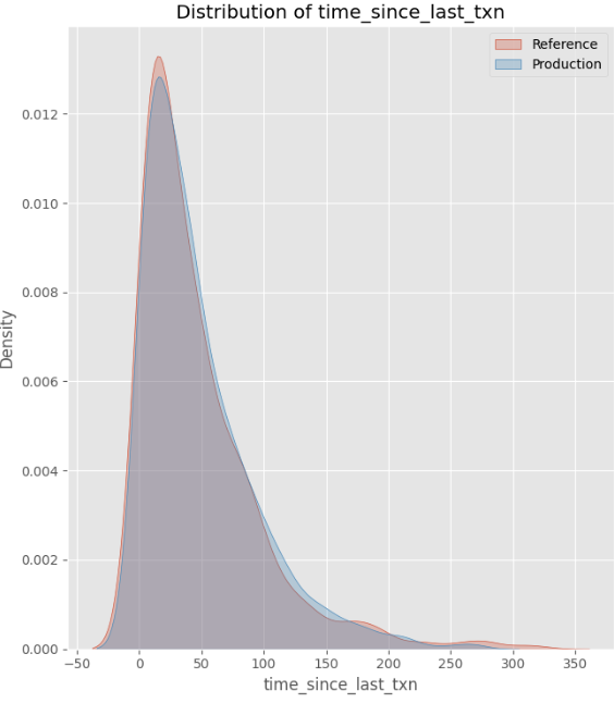
- Drifted features: Transaction Amount, Account Age, Transaction Count, and Entered PIN all experienced shifts in distribution, scale, or relationships.
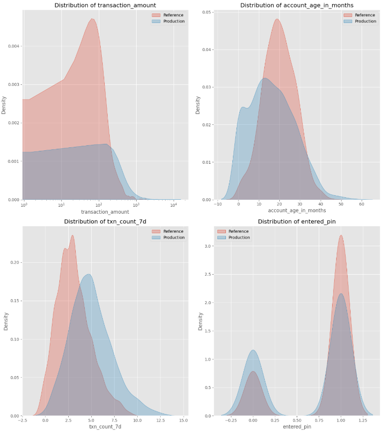
- Stable feature: Time Since Last Transaction remained unchanged.
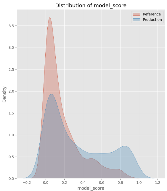
- Drifted scores: As a result of the drifted features, the distribution in model scores has also changed.
This setup allows us to analyze how feature drift impacts model scores in production.
Detecting model score drift using PSI
To monitor model scores, I used population stability index (PSI) to measure how much model score distribution has shifted over time.
PSI works by binning continuous model scores and comparing the proportion of scores in each bin between the reference and production datasets. It compares the differences in proportions and their logarithmic ratios to compute a single summary statistic to quantify the drift.
Python implementation:
# Define function to calculate PSI given two datasets
def calculate_psi(reference, production, bins=10):
  # Discretize scores into bins
  min_val, max_val = 0, 1
  bin_edges = np.linspace(min_val, max_val, bins + 1)

  # Calculate proportions in each bin
  ref_counts, _ = np.histogram(reference, bins=bin_edges)
  prod_counts, _ = np.histogram(production, bins=bin_edges)

  ref_proportions = ref_counts / len(reference)
  prod_proportions = prod_counts / len(production)

  # Avoid division by zero
  ref_proportions = np.clip(ref_proportions, 1e-8, 1)
  prod_proportions = np.clip(prod_proportions, 1e-8, 1)

  # Calculate PSI for each bin
  psi = np.sum((ref_proportions - prod_proportions) * np.log(ref_proportions / prod_proportions))

  return psi

# Calculate PSI
psi_value = calculate_psi(ref_data['model_score'], prod_data['model_score'], bins=10)
print(f"PSI Value: {psi_value}")
Below is a summary of how to interpret PSI values:
- PSI < 0.1: No drift, or very minor drift (distributions are almost identical).
- 0.1 ≤ PSI < 0.25: Some drift. The distributions are somewhat different.
- 0.25 ≤ PSI < 0.5: Moderate drift. A noticeable shift between the reference and production distributions.
- PSI ≥ 0.5: Significant drift. There is a large shift, indicating that the distribution in production has changed substantially from the reference data.
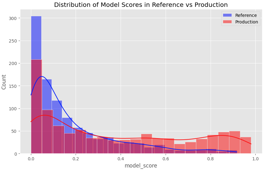
The PSI value of 0.6374 suggests a significant drift between our reference and production datasets. This aligns with the histogram of model score distributions, which visually confirms the shift towards higher scores in production — indicating an increase in risky transactions.
Detecting feature drift
Kolmogorov-Smirnov test for numeric features
The Kolmogorov-Smirnov (K-S) test is my preferred method for detecting drift in numeric features, because it is non-parametric, meaning it doesn’t assume a normal distribution.
The test compares a feature’s distribution in the reference and production datasets by measuring the maximum difference between the empirical cumulative distribution functions (ECDFs). The resulting K-S statistic ranges from 0 to 1:
- 0 indicates no difference between the two distributions.
- Values closer to 1 suggest a greater shift.
Python implementation:
# Create an empty dataframe
ks_results = pd.DataFrame(columns=['Feature', 'KS Statistic', 'p-value', 'Drift Detected'])

# Loop through all features and perform the K-S test
for col in numeric_cols:
    ks_stat, p_value = ks_2samp(ref_data[col], prod_data[col])
    drift_detected = p_value < 0.05

		# Store results in the dataframe
    ks_results = pd.concat([
        ks_results,
        pd.DataFrame({
            'Feature': [col],
            'KS Statistic': [ks_stat],
            'p-value': [p_value],
            'Drift Detected': [drift_detected]
        })
    ], ignore_index=True)
Below are ECDF charts of the four numeric features in our dataset:
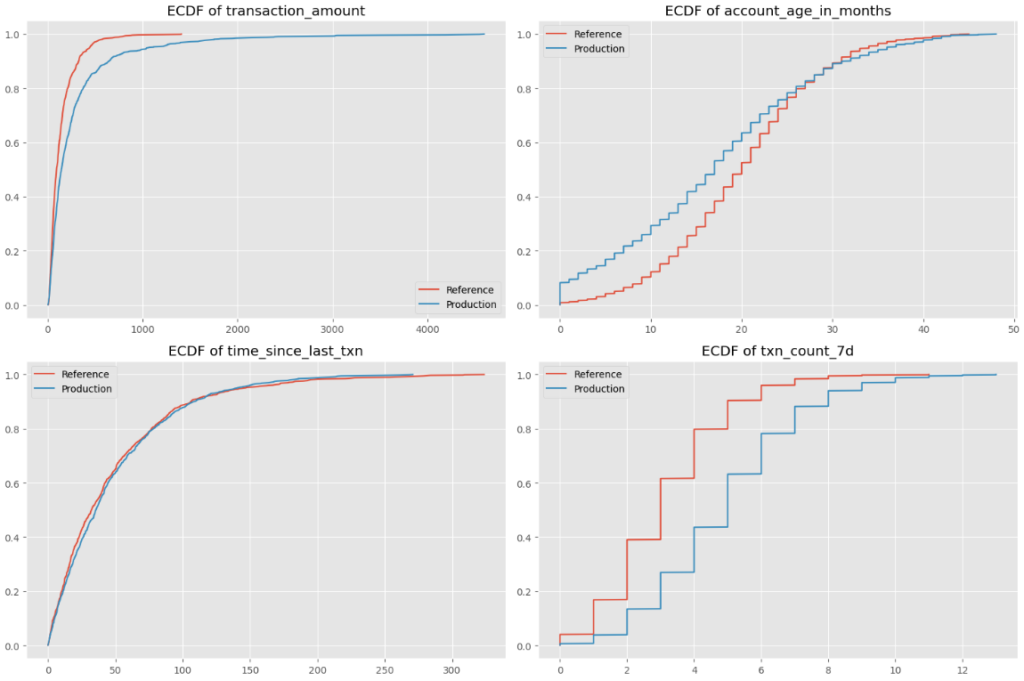
Let’s look at the account age feature as an example: the x-axis represents account age (0-50 months), while the y-axis shows the ECDF for both reference and production datasets. The production dataset skews towards newer accounts, as it has a larger proportion of observations have lower account ages.
Chi-Square test for categorical features
To detect shifts in categorical and boolean features, I like to use the Chi-Square test.
This test compares the frequency distribution of a categorical feature in the reference and production datasets, and returns two values:
- Chi-Square statistic: A higher value indicates a greater shift between the reference and production datasets.
- P-value: A p-value below 0.05 suggests that the difference between the reference and production datasets is statistically significant, indicating potential feature drift.
Python implementation:
# Create empty dataframe with corresponding column names
chi2_results = pd.DataFrame(columns=['Feature', 'Chi-Square Statistic', 'p-value', 'Drift Detected'])
for col in categorical_cols:
# Get normalized value counts for both reference and production datasets
ref_counts = ref_data[col].value_counts(normalize=True)
prod_counts = prod_data[col].value_counts(normalize=True)
# Ensure all categories are represented in both
all_categories = set(ref_counts.index).union(set(prod_counts.index))
ref_counts = ref_counts.reindex(all_categories, fill_value=0)
prod_counts = prod_counts.reindex(all_categories, fill_value=0)
# Create contingency table
contingency_table = np.array([ref_counts * len(ref_data), prod_counts * len(prod_data)])
# Perform Chi-Square test
chi2_stat, p_value, _, _ = chi2_contingency(contingency_table)
drift_detected = p_value < 0.05
# Store results in chi2_results dataframe
chi2_results = pd.concat([
chi2_results,
pd.DataFrame({
'Feature': [col],
'Chi-Square Statistic': [chi2_stat],
'p-value': [p_value],
'Drift Detected': [drift_detected]
})
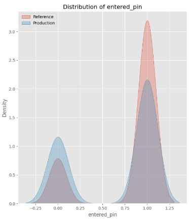
], ignore_index=True)The Chi-Square statistic of 57.31 with a p-value of 3.72e-14 confirms a large shift in our categorical feature, Entered PIN. This finding aligns with the histogram below, which visually illustrates the shift:
Detecting multivariate shifts
Spearman Correlation for shifts in pairwise interactions
In addition to monitoring individual feature shifts, it’s important to track shifts in relationships or interactions between features, known as multivariate shifts. Even if the distributions of individual features remain stable, multivariate shifts can signal meaningful differences in the data.
By default, Pandas’ .corr() function calculates Pearson correlation, which only captures linear relationships between variables. However, relationships between features are often non-linear yet still follow a consistent trend.
To capture this, we use Spearman correlation to measure monotonic relationships between features. It captures whether features change together in a consistent direction, even if their relationship isn’t strictly linear.
To assess shifts in feature relationships, we compare:
- Reference correlation (
ref_corr): Captures historical feature relationships in the reference dataset. - Production correlation (
prod_corr): Captures new feature relationships in production. - Absolute difference in correlation: Measures how much feature relationships have shifted between the reference and production datasets. Higher values indicate more significant shifts.
Python implementation:
# Calculate correlation matrices
ref_corr = ref_data.corr(method='spearman')
prod_corr = prod_data.corr(method='spearman')

# Calculate correlation difference
corr_diff = abs(ref_corr - prod_corr)
Example: Change in correlation
Now, let’s look at the correlation between transaction_amount and account_age_in_months:
- In
ref_corr, the correlation is 0.00095, indicating a weak relationship between the two features. - In
prod_corr, the correlation is -0.0325, indicating a weak negative correlation. - Absolute difference in the Spearman correlation is 0.0335, which is a small but noticeable shift.
The absolute difference in correlation indicates a shift in the relationship between transaction_amount and account_age_in_months.
There used to be no relationship between these two features, but the production dataset indicates that there is now a weak negative correlation, meaning that newer accounts have higher transaction accounts. This is spot on!
Autoencoder for complex, high-dimensional multivariate shifts
In addition to monitoring pairwise interactions, we can also look for shifts across more dimensions in the data.
Autoencoders are powerful tools for detecting high-dimensional multivariate shifts, where multiple features collectively change in ways that may not be apparent from looking at individual feature distributions or pairwise correlations.
An autoencoder is a neural network that learns a compressed representation of data through two components:
- Encoder: Compresses input data into a lower-dimensional representation.
- Decoder: Reconstructs the original input from the compressed representation.
To detect shifts, we compare the reconstructed output to the original input and compute the reconstruction loss.
- Low reconstruction loss → The autoencoder successfully reconstructs the data, meaning the new observations are similar to it has seen and learned.
- High reconstruction loss → The production data deviates significantly from the learned patterns, indicating potential drift.
Unlike traditional drift metrics that focus on individual features or pairwise relationships, autoencoders capture complex, non-linear dependencies across multiple variables simultaneously.
Python implementation:
ref_features = ref_data[numeric_cols + categorical_cols]
prod_features = prod_data[numeric_cols + categorical_cols]

# Normalize the data
scaler = StandardScaler()
ref_scaled = scaler.fit_transform(ref_features)
prod_scaled = scaler.transform(prod_features)

# Split reference data into train and validation
np.random.shuffle(ref_scaled)
train_size = int(0.8 * len(ref_scaled))
train_data = ref_scaled[:train_size]
val_data = ref_scaled[train_size:]

# Build autoencoder
input_dim = ref_features.shape[1]
encoding_dim = 3
# Input layer
input_layer = Input(shape=(input_dim, ))
# Encoder
encoded = Dense(8, activation="relu")(input_layer)
encoded = Dense(encoding_dim, activation="relu")(encoded)
# Decoder
decoded = Dense(8, activation="relu")(encoded)
decoded = Dense(input_dim, activation="linear")(decoded)
# Autoencoder
autoencoder = Model(input_layer, decoded)
autoencoder.compile(optimizer="adam", loss="mse")

# Train autoencoder
history = autoencoder.fit(
    train_data, train_data,
    epochs=50,
    batch_size=64,
    shuffle=True,
    validation_data=(val_data, val_data),
    verbose=0
)

# Calculate reconstruction error
ref_pred = autoencoder.predict(ref_scaled, verbose=0)
prod_pred = autoencoder.predict(prod_scaled, verbose=0)

ref_mse = np.mean(np.power(ref_scaled - ref_pred, 2), axis=1)
prod_mse = np.mean(np.power(prod_scaled - prod_pred, 2), axis=1)
The charts below show the distribution of reconstruction loss between both datasets.
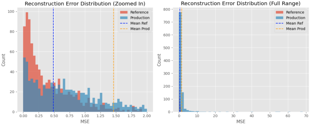
The production dataset has a higher mean reconstruction error than that of the reference dataset, indicating a shift in the overall data. This aligns with the changes in the production dataset with a higher number of newer accounts with high-value transactions.
Summarizing
Model monitoring is an essential, yet often overlooked, responsibility for data scientists and machine learning engineers.
All the statistical methods led to the same conclusion, which aligns with the observed shifts in the data: they detected a trend in production towards newer accounts making higher-value transactions. This shift resulted in higher model scores, signaling an increase in potential fraud.
In this post, I covered techniques for detecting drift on three different levels:
- Model score drift: Using Population Stability Index (PSI)
- Individual feature drift: Using Kolmogorov-Smirnov test for numeric features and Chi-Square test for categorical features
- Multivariate drift: Using Spearman correlation for pairwise interactions and autoencoders for high-dimensional, multivariate shifts.
These are just a few of the techniques I rely on for comprehensive monitoring — there are plenty of other equally valid statistical methods that can also detect drift effectively.
Detected shifts often point to underlying issues that warrant further investigation. The root cause could be as serious as a data collection bug, or as minor as a time change like daylight savings time adjustments.
There are also fantastic python packages, like evidently.ai, that automate many of these comparisons. However, I believe there’s significant value in deeply understanding the statistical techniques behind drift detection, rather than relying solely on these tools.
What’s the model monitoring process like at places you’ve worked?
Want to build your AI skills?
👉🏻 I run the AI Weekender and write weekly blog posts on data science, AI weekend projects, career advice for professionals in data.