In July 1959, Arthur Samuel developed one of the first agents to play the game of checkers. What constitutes an agent that plays checkers can be best described in Samuel’s own words, “…a computer [that] can be programmed so that it will learn to play a better game of checkers than can be played by the person who wrote the program” [1]. The checkers’ agent tries to follow the idea of simulating every possible move given the current situation and selecting the most advantageous one i.e. one that brings the player closer to winning. The move’s “advantageousness” is determined by an evaluation function, which the agent improves through experience. Naturally, the concept of an agent is not restricted to the game of checkers, and many practitioners have sought to match or surpass human performance in popular games. Notable examples include IBM’s Deep Blue (which managed to defeat Garry Kasparov, a chess world champion at the time), and Tesauro’s TD-Gammon, a temporal-difference approach, where the evaluation function was modelled using a neural network. In fact, TD-Gammon’s playing style was so uncommon that some experts even adopted some strategies it conjured up [2].
Unsurprisingly, research into creating such ‘agents’ only skyrocketed, with novel approaches able to reach peak human performance in complex games. In this post, we explore one such approach: the DQN approach introduced in 2013 by Mnih et al, in which playing Atari games is approached through a synthesis of Deep Neural Networks and TD-Learning (NB: the original paper came out in 2013, but we will focus on the 2015 version which comes with some technical improvements) [3, 4]. Before we continue, you should note that in the ever-expanding space of new approaches, DQN has been superseded by faster and more refined state-of-the-art methods. Yet, it remains an ideal stepping stone in the field of Deep Reinforcement Learning, widely recognized for combining deep learning with reinforcement learning. Hence, readers aiming to dive into Deep-RL are encouraged to begin with DQN.
This post is sectioned as follows: first, I define the problem with playing Atari games and explain why some traditional methods can be intractable. Finally, I present the specifics of the DQN approach and dive into the technical implementation.
The Problem At Hand
For the remainder of the post, I’ll assume that you know the basics of supervised learning, neural networks (basic FFNs and CNNs) and also basic reinforcement learning concepts (Bellman equations, TD-learning, Q-learning etc) If some of these RL concepts are foreign to you, then this playlist is a good introduction.
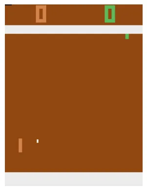
Atari is a nostalgia-laden term, featuring iconic games such as Pong, Breakout, Asteroids and many more. In this post, we restrict ourselves to Pong. Pong is a 2-player game, where each player controls a paddle and can use said paddle to hit the incoming ball. Points are scored when the opponent is unable to return the ball, in other words, the ball goes past them. A player wins when they reach 21 points.
Considering the sequential nature of the game, it might be appropriate to frame the problem as an RL problem, and then apply one of the solution methods. We can frame the game as an MDP:

The states would represent the current game state (where the ball or player paddle is etc, analogous to the idea of a search state). The rewards encapsulate our idea of winning and the actions correspond to the buttons on the Atari 2600 console. Our goal now becomes finding a policy

also known as the optimal policy. Let’s see what might happen if we try to train an agent using some classical RL algorithms.
A straightforward solution might entail solving the problem using a tabular approach. We could enumerate all states (and actions) and associate each state with a corresponding state or state-action value. We could then apply one of the classical RL methods (Monte-Carlo, TD-Learning, Value Iteration etc), taking a dynamic Programming approach. However, employing this approach faces large pitfalls rather quickly. What do we consider as states? How many states do we have to enumerate?
It quickly becomes quite difficult to answer these questions. Defining a state becomes difficult as many elements are in play when considering the idea of a state (i.e. the states need to be Markovian, encapsulate a search state etc). What about visual output (frames) to represent a state? After all this is how we as humans interact with Atari games. We see frames, deduce information regarding the game state and then choose the appropriate action. However, there are impossibly many states when using this representation, which would make our tabular approach quite intractable, memory-wise.
Now for the sake of argument imagine that we have enough memory to hold a table of this size. Even then we would need to explore all the states a good number of times to get good approximations of the value function. We would need to explore all possible states (or state-action) enough times to arrive at a useful value. Herein lies the runtime hurdle; it would be quite infeasible for the values to converge for all the states in the table in a reasonable amount of time as we have infinite states.
Perhaps instead of framing it as a reinforcement learning problem, can we instead rephrase it into a supervised learning problem? Perhaps a formulation in which the states are samples and the labels are the actions performed. Even this perspective brings forth new problems. Atari games are inherently sequential, each state is sampled based on the previous. This breaks the i.i.d assumptions applied in supervised learning, negatively affecting supervised learning-based solutions. Similarly, we would need to create a hand-labelled dataset, perhaps employing a human expert to hand label actions for each frame. This would be expensive and laborious, and still might yield insufficient results.
Solely relying on either supervised learning or RL may lead to inefficient learning, whether due to computational constraints or suboptimal policies. This calls for a more efficient approach to solving Atari games.
DQN: Intuition & Implementation
I assume you have some basic knowledge of PyTorch, Numpy and Python, though I’ll try to be as articulate as possible. For those unfamiliar, I recommend consulting: pytorch & numpy.
Deep-Q Networks aim to overcome the aforementioned barriers through a variety of techniques. Let’s go through each of the problems step-by-step and address how DQN mitigates or solves these challenges.
It’s quite hard to come up with a formal state definition for Atari games due to their diversity. DQN is designed to work for most Atari games, and as a result, we need a stated formalization that is compatible with said games. To this end, the visual representation (pixel values) of the games at any given moment are used to fashion a state. Naturally, this entails a continuous state space. This connects to our previous discussion on potential ways to represent states.
The challenge of continuous states is solved through function approximation. Function approximation (FA) aims to approximate the state-action value function directly using a function approximation. Let’s go through the steps to understand what the FA does.
Imagine that we have a network that given a state outputs the value of being in said state and performing a certain action. We then select actions based on the highest reward. However, this network would be short-sighted, only taking into account one timestep. Can we incorporate possible rewards from further down the line? Yes we can! This is the idea of the expected return. From this view, the FA becomes quite simple to understand; we aim to find a function:

In other words, a function which outputs the expected return of being in a given state after performing an action.
This idea of approximation becomes crucial due to the continuous nature of the state space. By using a FA, we can exploit the idea of generalization. States close to each other (similar pixel values) will have similar Q-values, meaning that we don’t need to cover the entire (infinite) state space, greatly lowering our computational overhead.
DQN employs FA in tandem with Q-learning. As a small refresher, Q-learning aims to find the expected return for being in a state and performing a certain action using bootstrapping. Bootstrapping models the expected return that we mentioned using the current Q-function. This ensures that we don’t need to wait till the end of an episode to update our Q-function. Q-learning is also 0ff-policy, which means that the data we use to learn the Q-function is different from the actual policy being learned. The resulting Q-function then corresponds to the optimal Q-function and can be used to find the optimal policy (just find the action that maximizes the Q-value in a given state). Moreover, Q-learning is a model-free solution, meaning that we don’t need to know the dynamics of the environment (transition functions etc) to learn an optimal policy, unlike in value iteration. Thus, DQN is also off-policy and model-free.
By using a neural network as our approximator, we need not construct a full table containing all the states and their respective Q-values. Our neural network will output the Q-value for being a given state and performing a certain action. From this point on, we refer to the approximator as the Q-network.
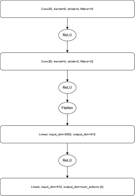
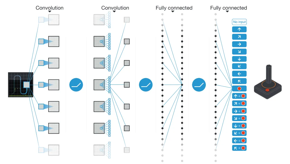
Since our states are defined by images, using a basic feed-forward network (FFN) would incur a large computational overhead. For this specific reason, we employ the use of a convolutional network, which is much better able to learn the distinct features of each state. The CNNs are able to distill the images down to a representation (this is the idea of representation learning), which is then fed to a FFN. The neural network architecture can be seen above. Instead of returning one value for:

we return an array with each value corresponding to a possible action in the given state (for Pong we can perform 6 actions, so we return 6 values).

Recall that to train a neural network we need to define a loss function that captures our goals. DQN uses the MSE loss function. For the predicted values we the output of our Q-network. For the true values, we use the bootstrapped values. Hence, our loss function becomes the following:

If we differentiate the loss function with respect to the weights we arrive at the following equation.

Plugging this into the stochastic gradient descent (SGD) equation, we arrive at Q-learning [4].
By performing SGD updates using the MSE loss function, we perform Q-learning. However, this is an approximation of Q-learning, as we don’t update on a single move but instead on a batch of moves. The expectation is simplified for expedience, though the message remains the same.
From another perspective, you can also think of the MSE loss function as nudging the predicted Q-values as close to the bootstrapped Q-values (after all this is what the MSE loss intends). This inadvertently mimics Q-learning, and slowly converges to the optimal Q-function.
By employing a function approximator, we become subject to the conditions of supervised learning, namely that the data is i.i.d. But in the case of Atari games (or MDPs) this condition is often not upheld. Samples from the environment are sequential in nature, making them dependent on each other. Similarly, as the agent improves the value function and updates its policy, the distribution from which we sample also changes, violating the condition of sampling from an identical distribution.
To solve this the authors of DQN capitalize on the idea of an experience replay. This concept is core to keep the training of DQN stable and convergent. An experience replay is a buffer which stores the tuple (s, a, r, s’, d) where s, a, r, s’ are returned after performing an action in an MDP, and d is a boolean representing whether the episode has finished or not. The replay has a maximum capacity which is defined beforehand. It might be simpler to think of the replay as a queue or a FIFO data structure; old samples are removed to make room for new samples. The experience replay is used to sample a random batch of tuples which are then used for training.
The experience replay helps with the alleviation of two major challenges when using neural network function approximators with RL problems. The first deals with the independence of the samples. By randomly sampling a batch of moves and then using those for training we decouple the training process from the sequential nature of Atari games. Each batch may have actions from different timesteps (or even different episodes), giving a stronger semblance of independence.
Secondly, the experience replay addresses the issue of non-stationarity. As the agent learns, changes in its behaviour are reflected in the data. This is the idea of non-stationarity; the distribution of data changes over time. By reusing samples in the replay and using a FIFO structure, we limit the adverse effects of non-stationarity on training. The distribution of the data still changes, but slowly and its effects are less impactful. Since Q-learning is an off-policy algorithm, we still end up learning the optimal policy, making this a viable solution. These changes allow for a more stable training procedure.
As a serendipitous side effect, the experience replay also allows for better data efficiency. Before training examples were discarded after being used for a single update step. However, through the use of an experience replay, we can reuse moves that we have made in the past for updates.
A change made in the 2015 Nature version of DQN was the introduction of a target network. Neural networks are fickle; slight changes in the weights can introduce drastic changes in the output. This is unfavourable for us, as we use the outputs of the Q-network to bootstrap our targets. If the targets are prone to large changes, it will destabilize training, which naturally we want to avoid. To alleviate this issue, the authors introduce a target network, which copies the weights of the Q-network every set amount of timesteps. By using the target network for bootstrapping, our bootstrapped targets are less unstable, making training more efficient.
Lastly, the DQN authors stack four consecutive frames after executing an action. This remark is made to ensure the Markovian property holds [9]. A singular frame omits many details of the game state such as the velocity and direction of the ball. A stacked representation is able to overcome these obstacles, providing a holistic view of the game at any given timestep.
With this, we have covered most of the major techniques used for training a DQN agent. Let’s go over the training procedure. The procedure will be more of an overview, and we’ll iron out the details in the implementation section.
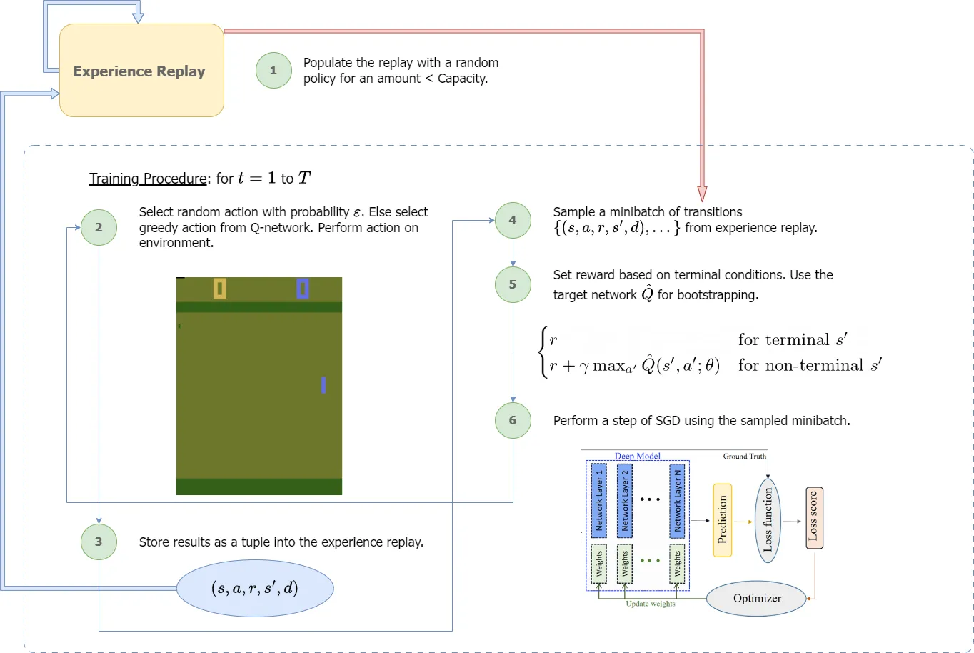
One important clarification arises from step 2. In this step, we perform a process called ε-greedy action selection. In ε-greedy, we randomly choose an action with probability ε, and otherwise choose the best possible action (according to our learned Q-network). Choosing an appropriate ε allows for the sufficient exploration of actions which is crucial to converge to a reliable Q-function. We often start with a high ε and slowly decay this value over time.
Implementation
If you want to follow along with my implementation of DQN then you will need the following libraries (apart from Numpy and PyTorch). I provide a concise explanation of their use.
- Arcade Learning Environment → ALE is a framework that allows us to interact with Atari 2600 environments. Technically we interface ALE through gymnasium, an API for RL environments and benchmarking.
- StableBaselines3 → SB3 is a deep reinforcement learning framework with a backend designed in Pytorch. We will only need this for some preprocessing wrappers.
Let’s import all of the necessary libraries.
import numpy as np
import time
import torch
import torch.nn as nn
import gymnasium as gym
import ale_py

from collections import deque # FIFO queue data structurefrom tqdm import tqdm  # progress barsfrom gymnasium.wrappers import FrameStack
from gymnasium.wrappers.frame_stack import LazyFrames
from stable_baselines3.common.atari_wrappers import (
  AtariWrapper,
  FireResetEnv,
)

gym.register_envs(ale_py) # we need to register ALE with gym

# use cuda if you have it otherwise cpu
device = 'cuda' if torch.cuda.is_available() else 'cpu'
device
First, we construct an environment, using the ALE framework. Since we are working with pong we create an environment with the name PongNoFrameskip-v4. With this, we can create an environment using the following code:
env = gym.make('PongNoFrameskip-v4', render_mode='rgb_array')The rgb_array parameter tells ALE to return pixel values instead of RAM codes (which is the default). The code to interact with the Atari becomes extremely simple with gym. The following excerpt encapsulates most of the utilities that we will need from gym.
# this code restarts/starts a environment to the beginning of an episode
observation, _ = env.reset()
for _ in range(100): # number of timesteps
# randomly get an action from possible actions
action = env.action_space.sample()
# take a step using the given action
# observation_prime refers to s', terminated and truncated refer to
# whether an episode has finished or been cut short
observation_prime, reward, terminated, truncated, _ = env.step(action)
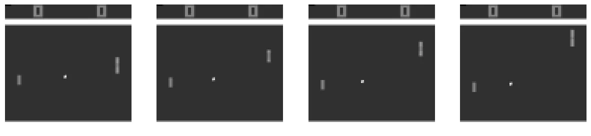
observation = observation_primeWith this, we are given states (we name them observations) with the shape (210, 160, 3). Hence the states are RGB images with the shape 210×160. An example can be seen in Figure 2. When training our DQN agent, an image of this size adds unnecessary computational overhead. A similar observation can be made about the fact that the frames are RGB (3 channels).
To solve this, we downsample the frame down to 84×84 and transform it into grayscale. We can do this by employing a wrapper from SB3, which does this for us. Now every time we perform an action our output will be in grayscale (with 1 channel) and of size 84×84.
env = AtariWrapper(env, terminal_on_life_loss=False, frame_skip=4)The wrapper above does more than downsample and turn our frame into grayscale. Let’s go over some other changes the wrapper introduces.
- Noop Reset → The start state of each Atari game is deterministic, i.e. you start at the same state each time the game ends. With this the agent may learn to memorize a sequence of actions from the starting state, resulting in a sub-optimal policy. To prevent this, we perform no actions for a set amount of timesteps in the beginning.
- Frame Skipping → In the ALE environment each frame needs an action. Instead of choosing an action at each frame, we select an action and repeat it for a set number of timesteps. This is the idea of frame skipping and allows for smoother transitions.
- Max-pooling → Due to the manner in which ALE/Atari renders its frames and the downsampling, it is possible that we encounter flickering. To solve this we take the max over two consecutive frames.
- Terminal Life on Loss → Many Atari games do not end when the player dies. Consider Pong, no player wins until the score hits 21. However, by default agents might consider the loss of life as the end of an episode, which is undesirable. This wrapper counteracts this and ends the episode when the game is truly over.
- Clip Reward → The gradients are highly sensitive to the magnitude of the rewards. To avoid unstable updates, we clip the rewards to be between {-1, 0, 1}.
Apart from these we also introduce an additional frame stack wrapper (FrameStack). This performs what was discussed above, stacking 4 frames on top of each to keep the states Markovian. The ALE environment returns LazyFrames, which are designed to be more memory efficient, as the same frame might occur multiple times. However, they are not compatible with many of the operations that we perform throughout the training procedure. To convert LazyFrames into usable objects, we apply a custom wrapper which converts an observation to Numpy before returning it to us. The code is shown below.
class LazyFramesToNumpyWrapper(gym.ObservationWrapper): # subclass obswrapper
  def __init__(self, env):
      super().__init__(env)
      self.env = env # the environment that we want to convert

  def observation(self, observation):
      # if its a LazyFrames object then turn it into a numpy array
      if isinstance(observation, LazyFrames):
          return np.array(observation)
      return observation
Let’s combine all of the wrappers into one function that returns an environment that does all of the above.
def make_env(game, render='rgb_array'):
  env = gym.make(game, render_mode=render)
  env = AtariWrapper(env, terminal_on_life_loss=False, frame_skip=4)
  env = FrameStack(env, num_stack=4)
  env = LazyFramesToNumpyWrapper(env)
  # sometimes a environment needs that the fire button be
  # pressed to start the game, this makes sure that game is started when needed
  if "FIRE" in env.unwrapped.get_action_meanings():
      env = FireResetEnv(env)
  return env
These changes are derived from the 2015 Nature paper and help to stabilize training [3]. The interfacing with gym remains the same as shown above. An example of the preprocessed states can be seen in Figure 7.
Now that we have an appropriate environment let’s move on to create the replay buffer.
class ReplayBuffer:

  def __init__(self, capacity, device):
      self.capacity = capacity
      self._buffer =  np.zeros((capacity,), dtype=object) # stores the tuples
      self._position = 0 # keep track of where we are
      self._size = 0
      self.device = device

  def store(self, experience):
      """Adds a new experience to the buffer,
        overwriting old entries when full."""
      idx = self._position % self.capacity # get the index to replace
      self._buffer[idx] = experience
      self._position += 1
      self._size = min(self._size + 1, self.capacity) # max size is the capacity

  def sample(self, batch_size):
      """ Sample a batch of tuples and load it onto the device
      """
      # if the buffer is not full capacity then return everything we have
      buffer = self._buffer[0:min(self._position-1, self.capacity-1)]
      # minibatch of tuples
      batch = np.random.choice(buffer, size=[batch_size], replace=True)

      # we need to return the objects as torch tensors, hence we delegate
      # this task to the transform function
      return (
          self.transform(batch, 0, shape=(batch_size, 4, 84, 84), dtype=torch.float32),
          self.transform(batch, 1, shape=(batch_size, 1), dtype=torch.int64),
          self.transform(batch, 2, shape=(batch_size, 1), dtype=torch.float32),
          self.transform(batch, 3, shape=(batch_size, 4, 84, 84), dtype=torch.float32),
          self.transform(batch, 4, shape=(batch_size, 1), dtype=torch.bool)
      )

  def transform(self, batch, index, shape, dtype):
      """ Transform a passed batch into a torch tensor for a given axis.
      E.g. if index 0 of a tuple means the state then we return all states
      as a torch tensor. We also return a specified shape.
      """
      # reshape the tensors as needed
      batched_values = np.array([val[index] for val in batch]).reshape(shape)
      # convert to torch tensors
      batched_values = torch.as_tensor(batched_values, dtype=dtype, device=self.device)
      return batched_values

  # below are some magic methods I used for debugging, not very important
  # they just turn the object into an arraylike object
  def __len__(self):
      return self._size

  def __getitem__(self, index):
      return self._buffer[index]

  def __setitem__(self, index, value: tuple):
      self._buffer[index] = value
The replay buffer works by allocating space in the memory for the given capacity. We maintain a pointer that keeps track of the number of objects added. Every time a new tuple is added we replace the oldest tuples with the new ones. To sample a minibatch, we first randomly sample a minibatch in numpy and then convert it into torch tensors, also loading it to the appropriate device.
Some of the aspects of the replay buffer are inspired by [8]. The replay buffer proved to be the biggest bottleneck in training the agent, and thus small speed-ups in the code proved to be monumentally important. An alternative strategy which uses an deque object to hold the tuples can also be used. If you are creating your own buffer, I would emphasize that you spend a little more time to ensure its efficiency.
We can now use this to create a function that creates a buffer and preloads a given number of tuples with a random policy.
def load_buffer(preload, capacity, game, *, device):
  # make the environment
  env = make_env(game)
  # create the buffer
  buffer = ReplayBuffer(capacity,device=device)

  # start the environment
  observation, _ = env.reset()
  # run for as long as the specified preload
  for _ in tqdm(range(preload)):
      # sample random action -> random policy
      action = env.action_space.sample()

      observation_prime, reward, terminated, truncated, _ = env.step(action)

      # store the results from the action as a python tuple object
      buffer.store((
          observation.squeeze(), # squeeze will remove the unnecessary grayscale channel
          action,
          reward,
          observation_prime.squeeze(),
          terminated or truncated))
      # set old observation to be new observation_prime
      observation = observation_prime

      # if the episode is done, then restart the environment
      done = terminated or truncated
      if done:
          observation, _ = env.reset()

  # return the env AND the loaded buffer
  return buffer, env
The function is quite straightforward, we create a buffer and environment object and then preload the buffer using a random policy. Note that we squeeze the observations to remove the redundant color channel. Let’s move on to the next step and define the function approximator.
class DQN(nn.Module):

  def __init__(
      self,
      env,
      in_channels = 4, # number of stacked frames
      hidden_filters = [16, 32],
      start_epsilon = 0.99, # starting epsilon for epsilon-decay
      max_decay = 0.1, # end epsilon-decay
      decay_steps = 1000, # how long to reach max_decay
      *args,
      **kwargs
  ) -> None:
      super().__init__(*args, **kwargs)

      # instantiate instance vars
      self.start_epsilon = start_epsilon
      self.epsilon = start_epsilon
      self.max_decay = max_decay
      self.decay_steps = decay_steps
      self.env = env
      self.num_actions = env.action_space.n

      # Sequential is an arraylike object that allows us to
      # perform the forward pass in one line
      self.layers = nn.Sequential(
          nn.Conv2d(in_channels, hidden_filters[0], kernel_size=8, stride=4),
          nn.ReLU(),
          nn.Conv2d(hidden_filters[0], hidden_filters[1], kernel_size=4, stride=2),
          nn.ReLU(),
          nn.Flatten(start_dim=1),
          nn.Linear(hidden_filters[1] * 9 * 9, 512), # the final value is calculated by using the equation for CNNs
          nn.ReLU(),
          nn.Linear(512, self.num_actions)
      )

      # initialize weights using he initialization
      # (pytorch already does this for conv layers but not linear layers)
      # this is not necessary and nothing you need to worry about
      self.apply(self._init)

  def forward(self, x):
      """ Forward pass. """
      # the /255.0 performs normalization of pixel values to be in [0.0, 1.0]
      return self.layers(x / 255.0)

  def epsilon_greedy(self, state, dim=1):
      """Epsilon greedy. Randomly select value with prob e,
        else choose greedy action"""

      rng = np.random.random() # get random value between [0, 1]

      if rng < self.epsilon: # for prob under e
          # random sample and return as torch tensor
          action = self.env.action_space.sample()
          action = torch.tensor(action)
      else:
          # use torch no grad to make sure no gradients are accumulated for this
          # forward pass
          with torch.no_grad():
              q_values = self(state)
          # choose best action
          action = torch.argmax(q_values, dim=dim)

      return action

  def epsilon_decay(self, step):
      # linearly decrease epsilon
      self.epsilon = self.max_decay + (self.start_epsilon - self.max_decay) * max(0, (self.decay_steps - step) / self.decay_steps)

  def _init(self, m):
    # initialize layers using he init
    if isinstance(m, (nn.Linear, nn.Conv2d)):
      nn.init.kaiming_normal_(m.weight, nonlinearity='relu')
      if m.bias is not None:
        nn.init.zeros_(m.bias)
That covers the model architecture. I used a linear ε-decay scheme, but feel free to try another. We can also create an auxiliary class that keeps track of important metrics. The class keeps track of rewards received for the last few episodes along with the respective lengths of said episodes.
class MetricTracker:
  def __init__(self, window_size=100):
      # the size of the history we use to track stats
      self.window_size = window_size
      self.rewards = deque(maxlen=window_size)
      self.current_episode_reward = 0

  def add_step_reward(self, reward):
      # add received reward to the current reward
      self.current_episode_reward += reward

  def end_episode(self):
      # add reward for episode to history
      self.rewards.append(self.current_episode_reward)
      # reset metrics
      self.current_episode_reward = 0

  # property just makes it so that we can return this value without
  # having to call it as a function
  @property
  def avg_reward(self):
      return np.mean(self.rewards) if self.rewards else 0
Great! Now we have everything we need to start training our agent. Let’s define the training function and go over how it works. Before that, we need to create the necessary objects to pass into our training function along with some hyperparameters. A small note: in the paper the authors use RMSProp, but instead we’ll use Adam. Adam proved to work for me with the given parameters, but you are welcome to try RMSProp or other variations.
TIMESTEPS = 6000000 # total number of timesteps for training
LR = 2.5e-4 # learning rate
BATCH_SIZE = 64 # batch size, change based on your hardware
C = 10000 # the interval at which we update the target network
GAMMA = 0.99 # the discount value
TRAIN_FREQ = 4 # in the paper the SGD updates are made every 4 actions
DECAY_START = 0 # when to start e-decay
FINAL_ANNEAL = 1000000 # when to stop e-decay

# load the buffer
buffer_pong, env_pong = load_buffer(50000, 150000, game='PongNoFrameskip-v4')

# create the networks, push the weights of the q_network onto the target network
q_network_pong = DQN(env_pong, decay_steps=FINAL_ANNEAL).to(device)
target_network_pong = DQN(env_pong, decay_steps=FINAL_ANNEAL).to(device)
target_network_pong.load_state_dict(q_network_pong.state_dict())

# create the optimizer
optimizer_pong = torch.optim.Adam(q_network_pong.parameters(), lr=LR)

# metrics class instantiation
metrics = MetricTracker()
def train(
env,
name, # name of the agent, used to save the agent
q_network,
target_network,
optimizer,
timesteps,
replay, # passed buffer
metrics, # metrics class
train_freq, # this parameter works complementary to frame skipping
batch_size,
gamma, # discount parameter
decay_start,
C,
save_step=850000, # I recommend setting this one high or else a lot of models will be saved
):
loss_func = nn.MSELoss() # create the loss object
start_time = time.time() # to check speed of the training procedure
episode_count = 0
best_avg_reward = -float('inf')
# reset the env
obs, _ = env.reset()
for step in range(1, timesteps+1): # start from 1 just for printing progress
# we need to pass tensors of size (batch_size, ...) to torch
# but the observation is just one so it doesn't have that dim
# so we add it artificially (step 2 in procedure)
batched_obs = np.expand_dims(obs.squeeze(), axis=0)
# perform e-greedy on the observation and convert the tensor into numpy and send it to the cpu
action = q_network.epsilon_greedy(torch.as_tensor(batched_obs, dtype=torch.float32, device=device)).cpu().item()
# take an action
obs_prime, reward, terminated, truncated, _ = env.step(action)
# store the tuple (step 3 in the procedure)
replay.store((obs.squeeze(), action, reward, obs_prime.squeeze(), terminated or truncated))
metrics.add_step_reward(reward)
obs = obs_prime
# train every 4 steps as per the paper
if step % train_freq == 0:
# sample tuples from the replay (step 4 in the procedure)
observations, actions, rewards, observation_primes, dones = replay.sample(batch_size)
# we don't want to accumulate gradients for this operation so use no_grad
with torch.no_grad():
q_values_minus = target_network(observation_primes)
# get the max over the target network
boostrapped_values = torch.amax(q_values_minus, dim=1, keepdim=True)
# this line basically makes so that for every sample in the minibatch which indicates
# that the episode is done, we return the reward, else we return the
# the bootstrapped reward (step 5 in the procedure)
y_trues = torch.where(dones, rewards, rewards + gamma * boostrapped_values)
y_preds = q_network(observations)
# compute the loss
# the gather gets the values of the q_network corresponding to the
# action taken
loss = loss_func(y_preds.gather(1, actions), y_trues)
# set the grads to 0, and perform the backward pass (step 6 in the procedure)
optimizer.zero_grad()
loss.backward()
optimizer.step()
# start the e-decay
if step > decay_start:
q_network.epsilon_decay(step)
target_network.epsilon_decay(step)
# if the episode is finished then we print some metrics
if terminated or truncated:
# compute steps per sec
elapsed_time = time.time() - start_time
steps_per_sec = step / elapsed_time
metrics.end_episode()
episode_count += 1
# reset the environment
obs, _ = env.reset()
# save a model if above save_step and if the average reward has improved
# this is kind of like early-stopping, but we don't stop we just save a model
if metrics.avg_reward > best_avg_reward and step > save_step:
best_avg_reward = metrics.avg_reward
torch.save({
'step': step,
'model_state_dict': q_network.state_dict(),
'optimizer_state_dict': optimizer.state_dict(),
'avg_reward': metrics.avg_reward,
}, f"models/{name}_dqn_best_{step}.pth")
# print some metrics
print(f"rStep: {step:,}/{timesteps:,} | "
f"Episodes: {episode_count} | "
f"Avg Reward: {metrics.avg_reward:.1f} | "
f"Epsilon: {q_network.epsilon:.3f} | "
f"Steps/sec: {steps_per_sec:.1f}", end="r")
# update the target network
if step % C == 0:
target_network.load_state_dict(q_network.state_dict())The training procedure closely follows Figure 6 and the algorithm described in the paper [4]. We first create the necessary objects such as the loss function etc and reset the environment. Then we can start the training loop, by using the Q-network to give us an action based on the ε-greedy policy. We simulate the environment one step forward using the action and push the resultant tuple onto the replay. If the update frequency condition is met, we can proceed with a training step. The motivation behind the update frequency element is something I am not 100% confident in. Currently, the explanation I can provide revolves around computational efficiency: training every 4 steps instead of every step majorly speeds up the algorithm and seems to work relatively well. In the update step itself, we sample a minibatch of tuples and run the model forward to produce predicted Q-values. We then create the target values (the bootstrapped true labels) using the piecewise function in step 5 in Figure 6. Performing an SGD step becomes quite straightforward from this point, since we can rely on autograd to compute the gradients and the optimizer to update the parameters.
If you followed along until now, you can use the following test function to test your saved model.
def test(game, model, num_eps=2):
  # render human opens an instance of the game so you can see it
  env_test = make_env(game, render='human')

  # load the model
  q_network_trained = DQN(env_test)
  q_network_trained.load_state_dict(torch.load(model, weights_only=False)['model_state_dict'])
  q_network_trained.eval() # set the model to inference mode (no gradients etc)
  q_network_trained.epsilon = 0.05 # a small amount of stochasticity


  rewards_list = []

  # run for set amount of episodes
  for episode in range(num_eps):
      print(f'Episode {episode}', end='r', flush=True)

      # reset the env
      obs, _ = env_test.reset()
      done = False
      total_reward = 0

      # until the episode is not done, perform the action from the q-network
      while not done:
          batched_obs = np.expand_dims(obs.squeeze(), axis=0)
          action = q_network_trained.epsilon_greedy(torch.as_tensor(batched_obs, dtype=torch.float32)).cpu().item()

          next_observation, reward, terminated, truncated, _ = env_test.step(action)
          total_reward += reward
          obs = next_observation

          done = terminated or truncated

      rewards_list.append(total_reward)

  # close the environment, since we use render human
  env_test.close()
  print(f'Average episode reward achieved: {np.mean(rewards_list)}')
Here’s how you can use it:
# make sure you use your latest model! I also renamed my model path so
# take that into account
test('PongNoFrameskip-v4', 'models/pong_dqn_best_6M.pth')
That’s everything for the code! You can see a trained agent below in Figure 8. It behaves quite similar to a human might play Pong, and is able to (consistently) beat the AI on the easiest difficulty. This naturally invites the question, how well does it perform on higher difficulties? Try it out using your own agent or my trained one!
An additional agent was trained on the game Breakout as well, the agent can be seen in Figure 9. Once again, I used the default mode and difficulty. It might be interesting to see how well it performs in different modes or difficulties.
Summary
DQN solves the issue of training agents to play Atari games. By using a FA, experience replay etc, we are able to train an agent that mimics or even surpasses human performance in Atari games [3]. Deep-RL agents can be finicky and you might have noticed that we use a lot of techniques to ensure that training is stable. If things are going wrong with your implementation it might not hurt to look at the details again.
If you want to check out the code for my implementation you can use this link. The repo also contains code to train your own model on the game of your choice (as long as it’s in ALE), as well as the trained weights for both Pong and Breakout.
I hope this was a helpful introduction to training DQN agents. To take things to the next level maybe you can try to tweak details to beat the higher difficulties. If you want to look further, there are many extensions to DQN you can explore, such as Dueling DQNs, Prioritized Replay etc.
References
[1] A. L. Samuel, “Some Studies in Machine Learning Using the Game of Checkers,” IBM Journal of Research and Development, vol. 3, no. 3, pp. 210–229, 1959. doi:10.1147/rd.33.0210.
[2] Sammut, Claude; Webb, Geoffrey I., eds. (2010), “TD-Gammon”, Encyclopedia of Machine Learning, Boston, MA: Springer US, pp. 955–956, doi:10.1007/978–0–387–30164–8_813, ISBN 978–0–387–30164–8, retrieved 2023–12–25
[3] Mnih, Volodymyr, Koray Kavukcuoglu, David Silver, Andrei A. Rusu, Joel Veness, Marc G. Bellemare, … and Demis Hassabis. “Human-Level Control through Deep Reinforcement Learning.” Nature 518, no. 7540 (2015): 529–533. https://doi.org/10.1038/nature14236
[4] Mnih, Volodymyr, Koray Kavukcuoglu, David Silver, Andrei A. Rusu, Joel Veness, Marc G. Bellemare, … and Demis Hassabis. “Playing Atari with Deep Reinforcement Learning.” arXiv preprint arXiv:1312.5602 (2013). https://arxiv.org/abs/1312.5602
[5] Sutton, Richard S., and Andrew G. Barto. Reinforcement Learning: An Introduction. 2nd ed., MIT Press, 2018.
[6] Russell, Stuart J., and Peter Norvig. Artificial Intelligence: A Modern Approach. 4th ed., Pearson, 2020.
[7] Goodfellow, I., Bengio, Y., & Courville, A. (2016). Deep Learning. MIT Press.
[8] Bailey, Jay. Deep Q-Networks Explained. 13 Sept. 2022, www.lesswrong.com/posts/kyvCNgx9oAwJCuevo/deep-q-networks-explained.
[9] Hausknecht, M., & Stone, P. (2015). Deep recurrent Q-learning for partially observable MDPs. arXiv preprint arXiv:1507.06527. https://arxiv.org/abs/1507.06527