1. Introduction

It’s pretty clear that most of our work will be automated by AI in the future. This will be possible because many researchers and professionals are working hard to make their work available online. These contributions not only help us understand fundamental concepts but also refine AI models, ultimately freeing up time to focus on other activities.

However, there is one concept that remains misunderstood, even among experts. It is spurious regression in time series analysis. This issue arises when regression models suggest strong relationships between variables, even when none exist. It is typically observed in time series regression equations that seem to have a high degree of fit — as indicated by a high R² (coefficient of multiple correlation) — but with an extremely low Durbin-Watson statistic (d), signaling strong autocorrelation in the error terms.

What is particularly surprising is that almost all econometric textbooks warn about the danger of autocorrelated errors, yet this issue persists in many published papers. Granger and Newbold (1974) identified several examples. For instance, they found published equations with R² = 0.997 and the Durbin-Watson statistic (d) equal to 0.53. The most extreme found is an equation with R² = 0.999 and d = 0.093.

It is especially problematic in economics and finance, where many key variables exhibit autocorrelation or serial correlation between adjacent values, particularly if the sampling interval is small, such as a week or a month, leading to misleading conclusions if not handled correctly. For example, today’s GDP is strongly correlated with the GDP of the previous quarter. Our post provides a detailed explanation of the results from Granger and Newbold (1974) and Python simulation (see section 7) replicating the key results presented in their article.

Whether you’re an economist, data scientist, or analyst working with time series data, understanding this issue is crucial to ensuring your models produce meaningful results.

To walk you through this paper, the next section will introduce the random walk and the ARIMA(0,1,1) process. In section 3, we will explain how Granger and Newbold (1974) describe the emergence of nonsense regressions, with examples illustrated in section 4. Finally, we’ll show how to avoid spurious regressions when working with time series data.

2. Simple presentation of a Random Walk and ARIMA(0,1,1) Process

2.1 Random Walk

Let 𝐗ₜ be a time series. We say that 𝐗ₜ follows a random walk if its representation is given by:

𝐗ₜ = 𝐗ₜ₋₁ + 𝜖ₜ. (1)

Where 𝜖ₜ is a white noise. It can be written as a sum of white noise, a useful form for simulation. It is a non-stationary time series because its variance depends on the time t.

2.2 ARIMA(0,1,1) Process

The ARIMA(0,1,1) process is given by:

𝐗ₜ = 𝐗ₜ₋₁ + 𝜖ₜ − 𝜃 𝜖ₜ₋₁. (2)

where 𝜖ₜ is a white noise. The ARIMA(0,1,1) process is non-stationary. It can be written as a sum of an independent random walk and white noise:

𝐗ₜ = 𝐗₀ + random walk + white noise. (3) This form is useful for simulation.

Those non-stationary series are often employed as benchmarks against which the forecasting performance of other models is judged.

3. Random walk can lead to Nonsense Regression

First, let’s recall the Linear Regression model. The linear regression model is given by:

𝐘 = 𝐗𝛽 + 𝜖. (4)

Where 𝐘 is a T × 1 vector of the dependent variable, 𝛽 is a K × 1 vector of the coefficients, 𝐗 is a T × K matrix of the independent variables containing a column of ones and (K−1) columns with T observations on each of the (K−1) independent variables, which are stochastic but distributed independently of the T × 1 vector of the errors 𝜖. It is generally assumed that:

𝐄(𝜖) = 0, (5)

and

𝐄(𝜖𝜖′) = 𝜎²𝐈. (6)

where 𝐈 is the identity matrix.

A test of the contribution of independent variables to the explanation of the dependent variable is the F-test. The null hypothesis of the test is given by:

𝐇₀: 𝛽₁ = 𝛽₂ = ⋯ = 𝛽ₖ₋₁ = 0, (7)

And the statistic of the test is given by:

𝐅 = (𝐑² / (𝐊−1)) / ((1−𝐑²) / (𝐓−𝐊)). (8)

where 𝐑² is the coefficient of determination.

If we want to construct the statistic of the test, let’s assume that the null hypothesis is true, and one tries to fit a regression of the form (Equation 4) to the levels of an economic time series. Suppose next that these series are not stationary or are highly autocorrelated. In such a situation, the test procedure is invalid since 𝐅 in (Equation 8) is not distributed as an F-distribution under the null hypothesis (Equation 7). In fact, under the null hypothesis, the errors or residuals from (Equation 4) are given by:

𝜖ₜ = 𝐘ₜ − 𝐗𝛽₀ ; t = 1, 2, …, T. (9)

And will have the same autocorrelation structure as the original series 𝐘.

Some idea of the distribution problem can arise in the situation when:

𝐘ₜ = 𝛽₀ + 𝐗ₜ𝛽₁ + 𝜖ₜ. (10)

Where 𝐘ₜ and 𝐗ₜ follow independent first-order autoregressive processes:

𝐘ₜ = 𝜌 𝐘ₜ₋₁ + 𝜂ₜ, and 𝐗ₜ = 𝜌* 𝐗ₜ₋₁ + 𝜈ₜ. (11)

Where 𝜂ₜ and 𝜈ₜ are white noise.

We know that in this case, 𝐑² is the square of the correlation between 𝐘ₜ and 𝐗ₜ. They use Kendall’s result from the article Knowles (1954), which expresses the variance of 𝐑:

𝐕𝐚𝐫(𝐑) = (1/T)* (1 + 𝜌𝜌*) / (1 − 𝜌𝜌*). (12)

Since 𝐑 is constrained to lie between -1 and 1, if its variance is greater than 1/3, the distribution of 𝐑 cannot have a mode at 0. This implies that 𝜌𝜌* > (T−1) / (T+1).

Thus, for example, if T = 20 and 𝜌 = 𝜌*, a distribution that is not unimodal at 0 will be obtained if 𝜌 > 0.86, and if 𝜌 = 0.9, 𝐕𝐚𝐫(𝐑) = 0.47. So the 𝐄(𝐑²) will be close to 0.47.

It has been shown that when 𝜌 is close to 1, 𝐑² can be very high, suggesting a strong relationship between 𝐘ₜ and 𝐗ₜ. However, in reality, the two series are completely independent. When 𝜌 is near 1, both series behave like random walks or near-random walks. On top of that, both series are highly autocorrelated, which causes the residuals from the regression to also be strongly autocorrelated. As a result, the Durbin-Watson statistic 𝐝 will be very low.

This is why a high 𝐑² in this context should never be taken as evidence of a true relationship between the two series.

To explore the possibility of obtaining a spurious regression when regressing two independent random walks, a series of simulations proposed by Granger and Newbold (1974) will be conducted in the next section.

4. Simulation results using Python.

In this section, we will show using simulations that using the regression model with independent random walks bias the estimation of the coefficients and the hypothesis tests of the coefficients are invalid. The Python code that will produce the results of the simulation will be presented in section 6.

A regression equation proposed by Granger and Newbold (1974) is given by:

𝐘ₜ = 𝛽₀ + 𝐗ₜ𝛽₁ + 𝜖ₜ

Where 𝐘ₜ and 𝐗ₜ were generated as independent random walks, each of length 50. The values 𝐒 = |𝛽̂₁| / √(𝐒𝐄̂(𝛽̂₁)), representing the statistic for testing the significance of 𝛽₁, for 100 simulations will be reported in the table below.

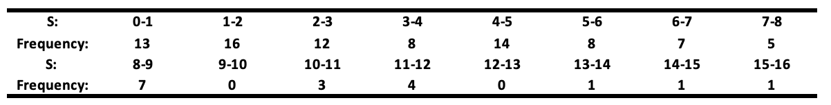
The null hypothesis of no relationship between 𝐘ₜ and 𝐗ₜ is rejected at the 5% level if 𝐒 > 2. This table shows that the null hypothesis (𝛽 = 0) is wrongly rejected in about a quarter (71 times) of all cases. This is awkward because the two variables are independent random walks, meaning there’s no actual relationship. Let’s break down why this happens.

If 𝛽̂₁ / 𝐒𝐄̂ follows a 𝐍(0,1), the expected value of 𝐒, its absolute value, should be √2 / π ≈ 0.8 (√2/π is the mean of the absolute value of a standard normal distribution). However, the simulation results show an average of 4.59, meaning the estimated 𝐒 is underestimated by a factor of:

4.59 / 0.8 = 5.7

In classical statistics, we usually use a t-test threshold of around 2 to check the significance of a coefficient. However, these results show that, in this case, you would need to use a threshold of 11.4 to properly test for significance:

2 × (4.59 / 0.8) = 11.4

Interpretation: We’ve just shown that including variables that don’t belong in the model — especially random walks — can lead to completely invalid significance tests for the coefficients.

To make their simulations even clearer, Granger and Newbold (1974) ran a series of regressions using variables that follow either a random walk or an ARIMA(0,1,1) process.

Here is how they set up their simulations:

They regressed a dependent series 𝐘ₜ on m series 𝐗ⱼ,ₜ (with j = 1, 2, …, m), varying m from 1 to 5. The dependent series 𝐘ₜ and the independent series 𝐗ⱼ,ₜ follow the same types of processes, and they tested four cases:

• Case 1 (Levels): 𝐘ₜ and 𝐗ⱼ,ₜ follow random walks.
• Case 2 (Differences): They use the first differences of the random walks, which are stationary.
• Case 3 (Levels): 𝐘ₜ and 𝐗ⱼ,ₜ follow ARIMA(0,1,1).
• Case 4 (Differences): They use the first differences of the previous ARIMA(0,1,1) processes, which are stationary.

Each series has a length of 50 observations, and they ran 100 simulations for each case.

All error terms are distributed as 𝐍(0,1), and the ARIMA(0,1,1) series are derived as the sum of the random walk and independent white noise. The simulation results, based on 100 replications with series of length 50, are summarized in the next table.

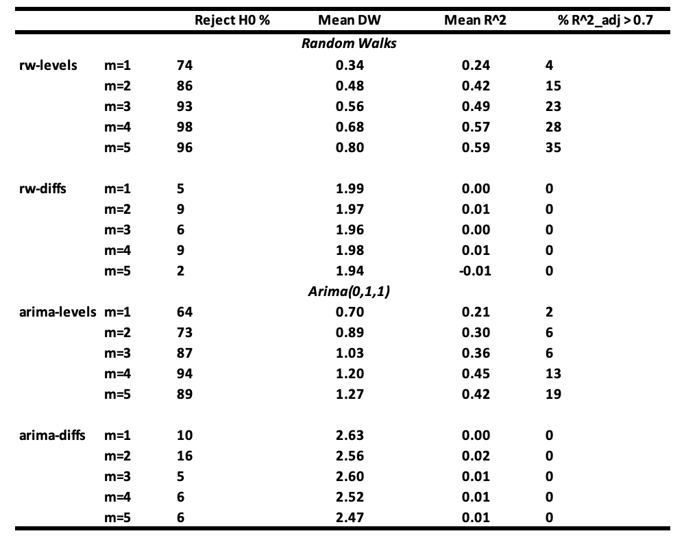
Interpretation of the results :

• It is seen that the probability of not rejecting the null hypothesis of no relationship between 𝐘ₜ and 𝐗ⱼ,ₜ becomes very small when m ≥ 3 when regressions are made with random walk series (rw-levels). The 𝐑² and the mean Durbin-Watson increase. Similar results are obtained when the regressions are made with ARIMA(0,1,1) series (arima-levels).
• When white noise series (rw-diffs) are used, classical regression analysis is valid since the error series will be white noise and least squares will be efficient.
• However, when the regressions are made with the differences of ARIMA(0,1,1) series (arima-diffs) or first-order moving average series MA(1) process, the null hypothesis is rejected, on average:

(10 + 16 + 5 + 6 + 6) / 5 = 8.6

which is greater than 5% of the time.

If your variables are random walks or close to them, and you include unnecessary variables in your regression, you will often get fallacious results. High 𝐑² and low Durbin-Watson values do not confirm a true relationship but instead indicate a likely spurious one.

5. How to avoid spurious regression in time series

It’s really hard to come up with a complete list of ways to avoid spurious regressions. However, there are a few good practices you can follow to minimize the risk as much as possible.

If one performs a regression analysis with time series data and finds that the residuals are strongly autocorrelated, there is a serious problem when it comes to interpreting the coefficients of the equation. To check for autocorrelation in the residuals, one can use the Durbin-Watson test or the Portmanteau test.

Based on the study above, we can conclude that if a regression analysis performed with economical variables produces strongly autocorrelated residuals, meaning a low Durbin-Watson statistic, then the results of the analysis are likely to be spurious, whatever the value of the coefficient of determination R² observed.

In such cases, it is important to understand where the mis-specification comes from. According to the literature, misspecification usually falls into three categories : (i) the omission of a relevant variable, (ii) the inclusion of an irrelevant variable, or (iii) autocorrelation of the errors. Most of the time, mis-specification comes from a mix of these three sources.

To avoid spurious regression in a time series, several recommendations can be made:

• The first recommendation is to select the right macroeconomic variables that are likely to explain the dependent variable. This can be done by reviewing the literature or consulting experts in the field.
• The second recommendation is to stationarize the series by taking first differences. In most cases, the first differences of macroeconomic variables are stationary and still easy to interpret. For macroeconomic data, it’s strongly recommended to differentiate the series once to reduce the autocorrelation of the residuals, especially when the sample size is small. There is indeed sometimes strong serial correlation observed in these variables. A simple calculation shows that the first differences will almost always have much smaller serial correlations than the original series.
• The third recommendation is to use the Box-Jenkins methodology to model each macroeconomic variable individually and then search for relationships between the series by relating the residuals from each individual model. The idea here is that the Box-Jenkins process extracts the explained part of the series, leaving the residuals, which contain only what can’t be explained by the series’ own past behavior. This makes it easier to check whether these unexplained parts (residuals) are related across variables.

6. Conclusion

Many econometrics textbooks warn about specification errors in regression models, but the problem still shows up in many published papers. Granger and Newbold (1974) highlighted the risk of spurious regressions, where you get a high paired with very low Durbin-Watson statistics.

Using Python simulations, we showed some of the main causes of these spurious regressions, especially including variables that don’t belong in the model and are highly autocorrelated. We also demonstrated how these issues can completely distort hypothesis tests on the coefficients.

Hopefully, this post will help reduce the risk of spurious regressions in future econometric analyses.

7. Appendice: Python code for simulation.

#####################################################Simulation Code for table 1 #####################################################

import numpy as np
import pandas as pd
import statsmodels.api as sm
import matplotlib.pyplot as plt

np.random.seed(123)
M = 100 
n = 50
S = np.zeros(M)
for i in range(M):
#---------------------------------------------------------------
# Generate the data
#---------------------------------------------------------------
    espilon_y = np.random.normal(0, 1, n)
    espilon_x = np.random.normal(0, 1, n)

    Y = np.cumsum(espilon_y)
    X = np.cumsum(espilon_x)
#---------------------------------------------------------------
# Fit the model
#---------------------------------------------------------------
    X = sm.add_constant(X)
    model = sm.OLS(Y, X).fit()
#---------------------------------------------------------------
# Compute the statistic
#------------------------------------------------------
    S[i] = np.abs(model.params[1])/model.bse[1]


#------------------------------------------------------ 
#              Maximum value of S
#------------------------------------------------------
S_max = int(np.ceil(max(S)))

#------------------------------------------------------ 
#                Create bins
#------------------------------------------------------
bins = np.arange(0, S_max + 2, 1)  

#------------------------------------------------------
#    Compute the histogram
#------------------------------------------------------
frequency, bin_edges = np.histogram(S, bins=bins)

#------------------------------------------------------
#    Create a dataframe
#------------------------------------------------------

df = pd.DataFrame({
    "S Interval": [f"{int(bin_edges[i])}-{int(bin_edges[i+1])}" for i in range(len(bin_edges)-1)],
    "Frequency": frequency
})
print(df)
print(np.mean(S))

#####################################################Simulation Code for table 2 #####################################################

import numpy as np
import pandas as pd
import statsmodels.api as sm
from statsmodels.stats.stattools import durbin_watson
from tabulate import tabulate

np.random.seed(1)  # Pour rendre les résultats reproductibles

#------------------------------------------------------
# Definition of functions
#------------------------------------------------------

def generate_random_walk(T):
    """
    Génère une série de longueur T suivant un random walk :
        Y_t = Y_{t-1} + e_t,
    où e_t ~ N(0,1).
    """
    e = np.random.normal(0, 1, size=T)
    return np.cumsum(e)

def generate_arima_0_1_1(T):
    """
    Génère un ARIMA(0,1,1) selon la méthode de Granger & Newbold :
    la série est obtenue en additionnant une marche aléatoire et un bruit blanc indépendant.
    """
    rw = generate_random_walk(T)
    wn = np.random.normal(0, 1, size=T)
    return rw + wn

def difference(series):
    """
    Calcule la différence première d'une série unidimensionnelle.
    Retourne une série de longueur T-1.
    """
    return np.diff(series)

#------------------------------------------------------
# Paramètres
#------------------------------------------------------

T = 50           # longueur de chaque série
n_sims = 100     # nombre de simulations Monte Carlo
alpha = 0.05     # seuil de significativité

#------------------------------------------------------
# Definition of function for simulation
#------------------------------------------------------

def run_simulation_case(case_name, m_values=[1,2,3,4,5]):
    """
    case_name : un identifiant pour le type de génération :
        - 'rw-levels' : random walk (levels)
        - 'rw-diffs'  : differences of RW (white noise)
        - 'arima-levels' : ARIMA(0,1,1) en niveaux
        - 'arima-diffs'  : différences d'un ARIMA(0,1,1) => MA(1)
    
    m_values : liste du nombre de régresseurs.
    
    Retourne un DataFrame avec pour chaque m :
        - % de rejets de H0
        - Durbin-Watson moyen
        - R^2_adj moyen
        - % de R^2 > 0.1
    """
    results = []
    
    for m in m_values:
        count_reject = 0
        dw_list = []
        r2_adjusted_list = []
        
        for _ in range(n_sims):
#--------------------------------------
# 1) Generation of independents de Y_t and X_{j,t}.
#----------------------------------------
            if case_name == 'rw-levels':
                Y = generate_random_walk(T)
                Xs = [generate_random_walk(T) for __ in range(m)]
            
            elif case_name == 'rw-diffs':
                # Y et X sont les différences d'un RW, i.e. ~ white noise
                Y_rw = generate_random_walk(T)
                Y = difference(Y_rw)
                Xs = []
                for __ in range(m):
                    X_rw = generate_random_walk(T)
                    Xs.append(difference(X_rw))
                # NB : maintenant Y et Xs ont longueur T-1
                # => ajuster T_effectif = T-1
                # => on prendra T_effectif points pour la régression
            
            elif case_name == 'arima-levels':
                Y = generate_arima_0_1_1(T)
                Xs = [generate_arima_0_1_1(T) for __ in range(m)]
            
            elif case_name == 'arima-diffs':
                # Différences d'un ARIMA(0,1,1) => MA(1)
                Y_arima = generate_arima_0_1_1(T)
                Y = difference(Y_arima)
                Xs = []
                for __ in range(m):
                    X_arima = generate_arima_0_1_1(T)
                    Xs.append(difference(X_arima))
            
            # 2) Prépare les données pour la régression
            #    Selon le cas, la longueur est T ou T-1
            if case_name in ['rw-levels','arima-levels']:
                Y_reg = Y
                X_reg = np.column_stack(Xs) if m>0 else np.array([])
            else:
                # dans les cas de différences, la longueur est T-1
                Y_reg = Y
                X_reg = np.column_stack(Xs) if m>0 else np.array([])
            
            # 3) Régression OLS
            X_with_const = sm.add_constant(X_reg)  # Ajout de l'ordonnée à l'origine
            model = sm.OLS(Y_reg, X_with_const).fit()
            
            # 4) Test global F : H0 : tous les beta_j = 0
            #    On regarde si p-value < alpha
            if model.f_pvalue is not None and model.f_pvalue  0.7)
        
        results.append({
            'm': m,
            'Reject %': reject_percent,
            'Mean DW': dw_mean,
            'Mean R^2': r2_mean,
            '% R^2_adj>0.7': r2_above_0_7_percent
        })
    
    return pd.DataFrame(results)
    
#------------------------------------------------------
# Application of the simulation
#------------------------------------------------------       

cases = ['rw-levels', 'rw-diffs', 'arima-levels', 'arima-diffs']
all_results = {}

for c in cases:
    df_res = run_simulation_case(c, m_values=[1,2,3,4,5])
    all_results[c] = df_res

#------------------------------------------------------
# Store data in table
#------------------------------------------------------

for case, df_res in all_results.items():
    print(f"nn{case}")
    print(tabulate(df_res, headers='keys', tablefmt='fancy_grid'))

References

• Granger, Clive WJ, and Paul Newbold. 1974. “Spurious Regressions in Econometrics.” Journal of Econometrics 2 (2): 111–20.
• Knowles, EAG. 1954. “Exercises in Theoretical Statistics.” Oxford University Press.