Let’s say you are in a customer care center, and you would like to know the probability distribution of the number of calls per minute, or in other words, you want to answer the question: what is the probability of receiving zero, one, two, … etc., calls per minute? You need this distribution in order to predict the probability of receiving different number of calls based on which you can plan how many employees are needed, whether or not an expansion is required, etc.

In order to let our decision ‘data informed’ we start by collecting data from which we try to infer this distribution, or in other words, we want to generalize from the sample data to the unseen data which is also known as the population in statistical terms. This is the essence of statistical inference.

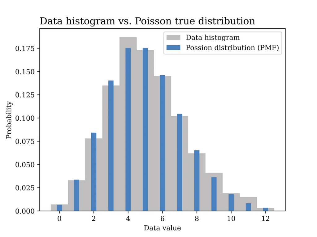
From the collected data we can compute the relative frequency of each value of calls per minute. For example, if the collected data over time looks something like this: 2, 2, 3, 5, 4, 5, 5, 3, 6, 3, 4, … etc. This data is obtained by counting the number of calls received every minute. In order to compute the relative frequency of each value you can count the number of occurrences of each value divided by the total number of occurrences. This way you will end up with something like the grey curve in the below figure, which is equivalent to the histogram of the data in this example.

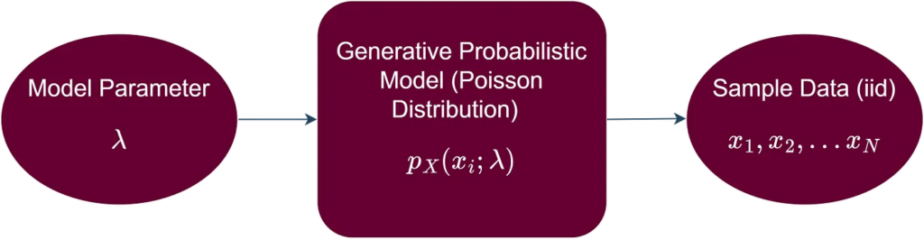
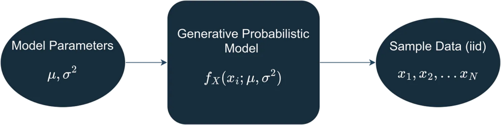
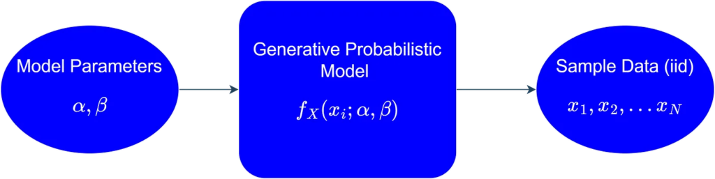
Another option is to assume that each data point from our data is a realization of a random variable (X) that follows a certain probability distribution. This probability distribution represents all the possible values that are generated if we were to collect this data long into the future, or in other words, we can say that it represents the population from which our sample data was collected. Furthermore, we can assume that all the data points come from the same probability distribution, i.e., the data points are identically distributed. Moreover, we assume that the data points are independent, i.e., the value of one data point in the sample is not affected by the values of the other data points. The independence and identical distribution (iid) assumption of the sample data points allows us to proceed mathematically with our statistical inference problem in a systematic and straightforward way. In more formal terms, we assume that a generative probabilistic model is responsible for generating the iid data as shown below.

In this particular example, a Poisson distribution with mean value λ = 5 is assumed to have generated the data as shown in the blue curve in the below figure. In other words, we assume here that we know the true value of λ which is generally not known and needs to be estimated from the data.

As opposed to the previous method in which we had to compute the relative frequency of each value of calls per minute (e.g., 12 values to be estimated in this example as shown in the grey figure above), now we only have one parameter that we aim at finding which is λ. Another advantage of this generative model approach is that it is better in terms of generalization from sample to population. The assumed probability distribution can be said to have summarized the data in an elegant way that follows the Occam’s razor principle.

Before proceeding further into how we aim at finding this parameter λ, let’s show some Python code first that was used to generate the above figure.

# Import the Python libraries that we will need in this article
import pandas as pd
import matplotlib.pyplot as plt
import numpy as np
import seaborn as sns
import math
from scipy import stats

# Poisson distribution example
lambda_ = 5
sample_size = 1000
data_poisson = stats.poisson.rvs(lambda_,size= sample_size) # generate data

# Plot the data histogram vs the PMF
x1 = np.arange(data_poisson.min(), data_poisson.max(), 1)
fig1, ax = plt.subplots()
plt.bar(x1, stats.poisson.pmf(x1,lambda_),
        label="Possion distribution (PMF)",color = BLUE2,linewidth=3.0,width=0.3,zorder=2)
ax.hist(data_poisson, bins=x1.size, density=True, label="Data histogram",color = GRAY9, width=1,zorder=1,align='left')

ax.set_title("Data histogram vs. Poisson true distribution", fontsize=14, loc='left')
ax.set_xlabel('Data value')
ax.set_ylabel('Probability')
ax.legend()
plt.savefig("Possion_hist_PMF.png", format="png", dpi=800)

Our problem now is about estimating the value of the unknown parameter λ using the data we collected. This is where we will use the method of moments (MoM) approach that appears in the title of this article.

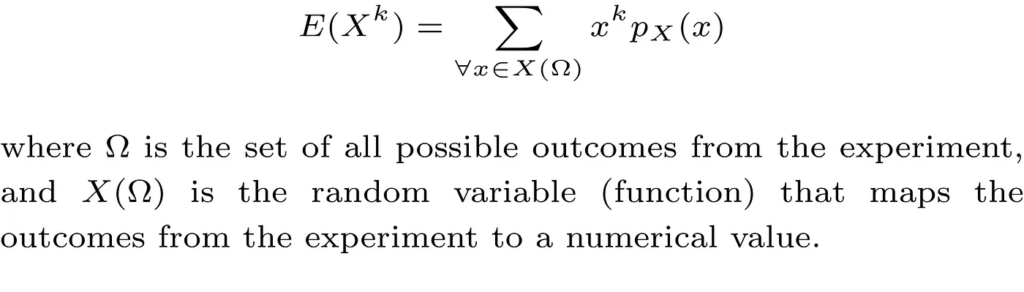
First, we need to define what is meant by the moment of a random variable. Mathematically, the kth moment of a discrete random variable (X) is defined as follows:

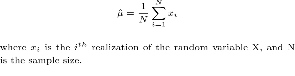
Take the first moment E(X) as an example, which is also the mean μ of the random variable, and assuming that we collect our data which is modeled as N iid realizations of the random variable X. A reasonable estimate of μ is the sample mean which is defined as follows:

Thus, in order to obtain a MoM estimate of a model parameter that parametrizes the probability distribution of the random variable X, we first write the unknown parameter as a function of one or more of the kth moments of the random variable, then we replace the kth moment with its sample estimate. The more unknown parameters we have in our models, the more moments we need.

In our Poisson model example, this is very simple as shown below.

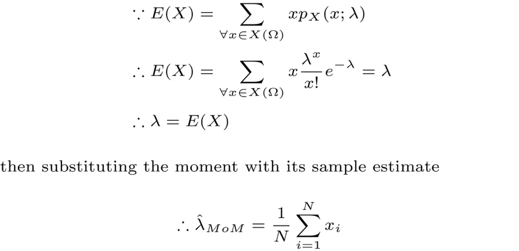
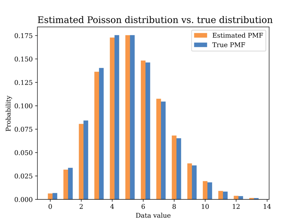
In the next part, we test our MoM estimator on the simulated data we had earlier. The Python code for obtaining the estimator and plotting the corresponding probability distribution using the estimated parameter is shown below.

# Method of moments estimator using the data (Poisson Dist)
lambda_hat = sum(data_poisson) / len(data_poisson)

# Plot the MoM estimated PMF vs the true PMF
x1 = np.arange(data_poisson.min(), data_poisson.max(), 1)
fig2, ax = plt.subplots()
plt.bar(x1, stats.poisson.pmf(x1,lambda_hat),
        label="Estimated PMF",color = ORANGE1,linewidth=3.0,width=0.3)
plt.bar(x1+0.3, stats.poisson.pmf(x1,lambda_),
        label="True PMF",color = BLUE2,linewidth=3.0,width=0.3)

ax.set_title("Estimated Poisson distribution vs. true distribution", fontsize=14, loc='left')
ax.set_xlabel('Data value')
ax.set_ylabel('Probability')
ax.legend()
#ax.grid()
plt.savefig("Possion_true_vs_est.png", format="png", dpi=800)

The below figure shows the estimated distribution versus the true distribution. The distributions are quite close indicating that the MoM estimator is a reasonable estimator for our problem. In fact, replacing expectations with averages in the MoM estimator implies that the estimator is a consistent estimator by the law of large numbers, which is a good justification for using such estimator.

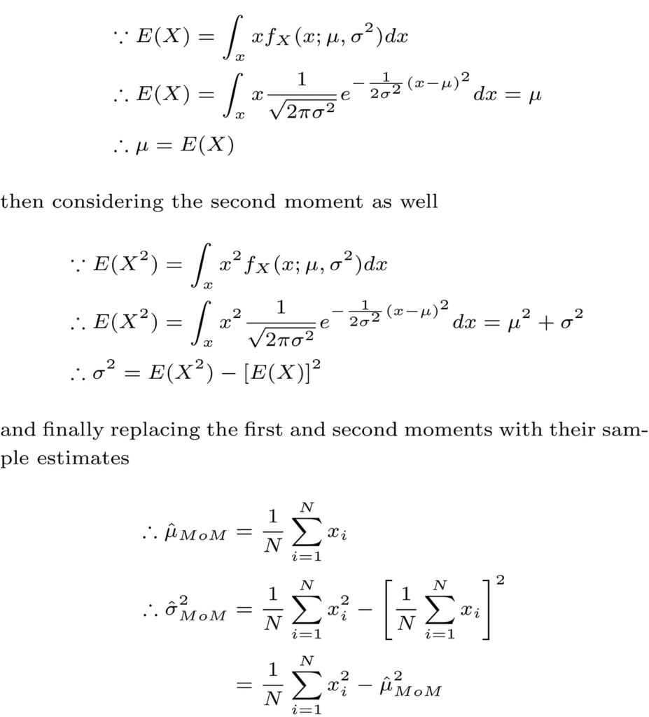
Another MoM estimation example is shown below assuming the iid data is generated by a normal distribution with mean μ and variance σ² as shown below.

In this particular example, a Gaussian (normal) distribution with mean value μ = 10 and σ = 2 is assumed to have generated the data. The histogram of the generated data sample (sample size = 1000) is shown in grey in the below figure, while the true distribution is shown in the blue curve.

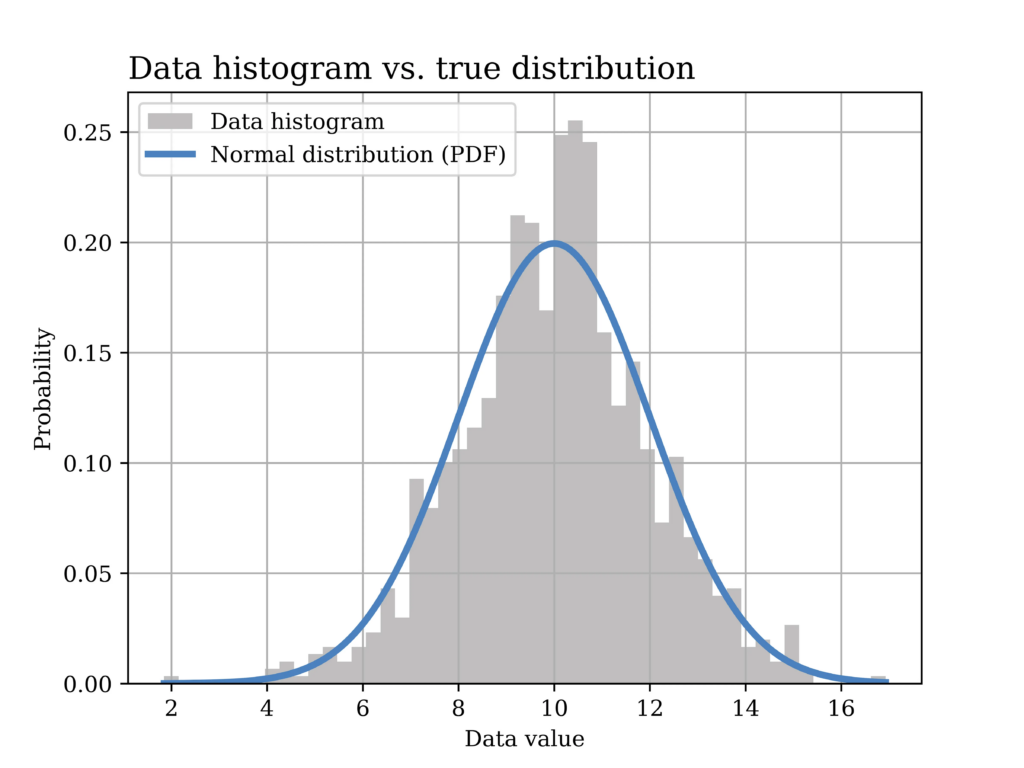
The Python code that was used to generate the above figure is shown below.

# Normal distribution example
mu = 10
sigma = 2
sample_size = 1000
data_normal = stats.norm.rvs(loc=mu, scale=sigma ,size= sample_size) # generate data

# Plot the data histogram vs the PDF
x2 = np.linspace(data_normal.min(), data_normal.max(), sample_size)
fig3, ax = plt.subplots()
ax.hist(data_normal, bins=50, density=True, label="Data histogram",color = GRAY9)
ax.plot(x2, stats.norm(loc=mu, scale=sigma).pdf(x2),
        label="Normal distribution (PDF)",color = BLUE2,linewidth=3.0)

ax.set_title("Data histogram vs. true distribution", fontsize=14, loc='left')
ax.set_xlabel('Data value')
ax.set_ylabel('Probability')
ax.legend()
ax.grid()

plt.savefig("Normal_hist_PMF.png", format="png", dpi=800)

Now, we would like to use the MoM estimator to find an estimate of the model parameters, i.e., μ and σ² as shown below.

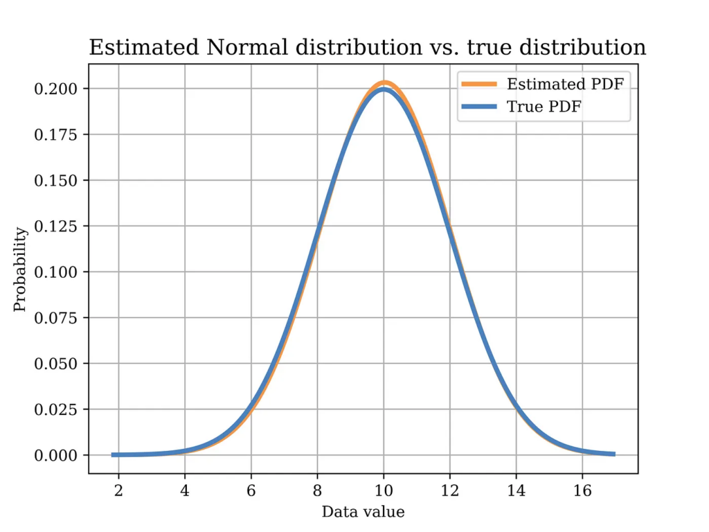
In order to test this estimator using our sample data, we plot the distribution with the estimated parameters (orange) in the below figure, versus the true distribution (blue). Again, it can be shown that the distributions are quite close. Of course, in order to quantify this estimator, we need to test it on multiple realizations of the data and observe properties such as bias, variance, etc. Such important aspects have been discussed in an earlier article.

The Python code that was used to estimate the model parameters using MoM, and to plot the above figure is shown below.

# Method of moments estimator using the data (Normal Dist)
mu_hat = sum(data_normal) / len(data_normal) # MoM mean estimator
var_hat = sum(pow(x-mu_hat,2) for x in data_normal) / len(data_normal) # variance
sigma_hat = math.sqrt(var_hat)  # MoM standard deviation estimator

# Plot the MoM estimated PDF vs the true PDF
x2 = np.linspace(data_normal.min(), data_normal.max(), sample_size)
fig4, ax = plt.subplots()
ax.plot(x2, stats.norm(loc=mu_hat, scale=sigma_hat).pdf(x2),
        label="Estimated PDF",color = ORANGE1,linewidth=3.0)
ax.plot(x2, stats.norm(loc=mu, scale=sigma).pdf(x2),
        label="True PDF",color = BLUE2,linewidth=3.0)

ax.set_title("Estimated Normal distribution vs. true distribution", fontsize=14, loc='left')
ax.set_xlabel('Data value')
ax.set_ylabel('Probability')
ax.legend()
ax.grid()
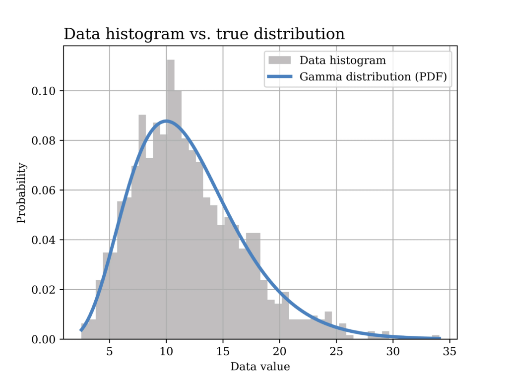
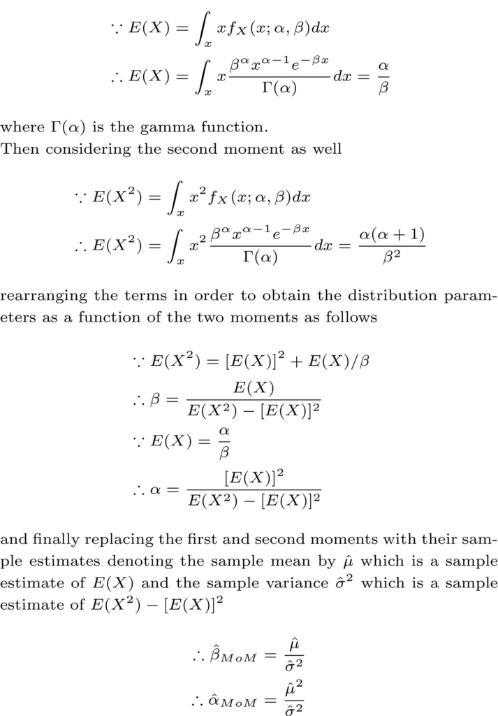
plt.savefig("Normal_true_vs_est.png", format="png", dpi=800)

Another useful probability distribution is the Gamma distribution. An example for the application of this distribution in real life was discussed in a previous article. However, in this article, we derive the MoM estimator of the Gamma distribution parameters α and β as shown below, assuming the data is iid.

In this particular example, a Gamma distribution with α = 6 and β = 0.5 is assumed to have generated the data. The histogram of the generated data sample (sample size = 1000) is shown in grey in the below figure, while the true distribution is shown in the blue curve.

The Python code that was used to generate the above figure is shown below.

# Gamma distribution example
alpha_ = 6 # shape parameter
scale_ = 2 # scale paramter (lamda) = 1/beta in gamma dist.
sample_size = 1000
data_gamma = stats.gamma.rvs(alpha_,loc=0, scale=scale_ ,size= sample_size) # generate data

# Plot the data histogram vs the PDF
x3 = np.linspace(data_gamma.min(), data_gamma.max(), sample_size)
fig5, ax = plt.subplots()
ax.hist(data_gamma, bins=50, density=True, label="Data histogram",color = GRAY9)
ax.plot(x3, stats.gamma(alpha_,loc=0, scale=scale_).pdf(x3),
        label="Gamma distribution (PDF)",color = BLUE2,linewidth=3.0)

ax.set_title("Data histogram vs. true distribution", fontsize=14, loc='left')
ax.set_xlabel('Data value')
ax.set_ylabel('Probability')
ax.legend()
ax.grid()
plt.savefig("Gamma_hist_PMF.png", format="png", dpi=800)

Now, we would like to use the MoM estimator to find an estimate of the model parameters, i.e., α and β, as shown below.

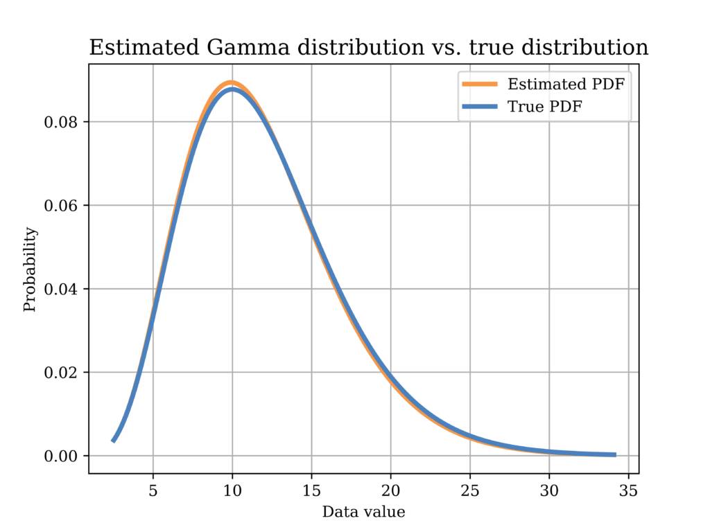
In order to test this estimator using our sample data, we plot the distribution with the estimated parameters (orange) in the below figure, versus the true distribution (blue). Again, it can be shown that the distributions are quite close.

The Python code that was used to estimate the model parameters using MoM, and to plot the above figure is shown below.

# Method of moments estimator using the data (Gamma Dist)
sample_mean = data_gamma.mean()
sample_var = data_gamma.var()
scale_hat = sample_var/sample_mean #scale is equal to 1/beta in gamma dist.
alpha_hat = sample_mean**2/sample_var

# Plot the MoM estimated PDF vs the true PDF
x4 = np.linspace(data_gamma.min(), data_gamma.max(), sample_size)
fig6, ax = plt.subplots()

ax.plot(x4, stats.gamma(alpha_hat,loc=0, scale=scale_hat).pdf(x4),
        label="Estimated PDF",color = ORANGE1,linewidth=3.0)
ax.plot(x4, stats.gamma(alpha_,loc=0, scale=scale_).pdf(x4),
        label="True PDF",color = BLUE2,linewidth=3.0)

ax.set_title("Estimated Gamma distribution vs. true distribution", fontsize=14, loc='left')
ax.set_xlabel('Data value')
ax.set_ylabel('Probability')
ax.legend()
ax.grid()
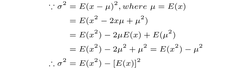
plt.savefig("Gamma_true_vs_est.png", format="png", dpi=800)

Note that we used the following equivalent ways of writing the variance when deriving the estimators in the cases of Gaussian and Gamma distributions.

Conclusion

In this article, we explored various examples of the method of moments estimator and its applications in different problems in data science. Moreover, detailed Python code that was used to implement the estimators from scratch as well as to plot the different figures is also shown. I hope that you will find this article helpful.