This is Part 2 of an exploration into the unexpected quirks of programming the Raspberry Pi Pico PIO with Micropython. If you missed Part 1, we uncovered four Wats that challenge assumptions about register count, instruction slots, the behavior of pull noblock, and smart yet cheap hardware.
Now, we continue our journey toward crafting a theremin-like musical instrument — a project that reveals some of the quirks and perplexities of PIO programming. Prepare to challenge your understanding of constants in a way that brings to mind a Shakespearean tragedy.
Wat 5: Inconstant constants
In the world of PIO programming, constants should be reliable, steadfast, and, well, constant. But what if they’re not? This brings us to a puzzling Wat about how the set instruction in PIO works—or doesn’t—when handling larger constants.
Much like Juliet doubting Romeo’s constancy, you might find yourself wondering if PIO constants will, as she says, “prove likewise variable.”
The problem: Constants are not as big as they seem
Imagine you’re programming an ultrasonic range finder and need to count down from 500 while waiting for the Echo signal to drop from high to low. To set up this wait time in PIO, you might naïvely try to load the constant value directly using set:
; In Rust, be sure 'config.shift_in.direction = ShiftDirection::Left;'
set y, 15       ; Load upper 5 bits (0b01111)
mov isr, y      ; Transfer to ISR (clears ISR)
set y, 20       ; Load lower 5 bits (0b10100)
in y, 5         ; Shift in lower bits to form 500 in ISR
mov y, isr      ; Transfer back to y
Aside: Don’t try to understand the crazy jmp operations here. We’ll discuss those next in Wat 6.
But here’s the tragic twist: the set instruction in PIO is limited to constants between 0 and 31. Moreover, the star-crossed set instruction doesn’t report an error. Instead, it silently corrupts the entire PIO instruction. This produces a nonsense result.
Workarounds for inconstant constants
To address this limitation, consider the following approaches:
- Read Values and Store Them in a Register: We saw this approach in Wat 1. You can load your constant in the
osrregister, then transfer it to y. For example:
# Read the max echo wait into OSR.
pull                    ; same as pull block
mov y, osr ; Load max echo wait into Y- Shift and Combine Smaller Values: Using the isr register and the in instruction, you can build up a constant of any size. This, however, consumes time and operations from your 32-operation budget (see Part 1, Wat 2).
; In Rust, be sure 'config.shift_in.direction = ShiftDirection::Left;'

set y, 15       ; Load upper 5 bits (0b01111)
mov isr, y      ; Transfer to ISR (clears ISR)
set y, 20       ; Load lower 5 bits (0b10100)
in y, 5         ; Shift in lower bits to form 500 in ISR
mov y, isr ; Transfer back to y- Slow Down the Timing: Reduce the frequency of the state machine to stretch delays over more system clock cycles. For example, lowering the state machine speed from 125 MHz to 343 kHz reduces the timeout constant
182,216to500. - Use Extra Delays and (Nested) Loops: All instructions support an optional delay, allowing you to add up to 31 extra cycles. (To generate even longer delays, use loops — or even nested loops.)
; Generate 10μs trigger pulse (4 cycles at 343_000Hz)
set pins, 1 [3]       ; Set trigger pin to high, add delay of 3
set pins, 0 ; Set trigger pin to low voltage- Use the “Subtraction Trick” to Generate the Maximum 32-bit Integer: In Wat 7, we’ll explore a way to generate
4,294,967,295(the maximum unsigned 32-bit integer) via subtraction.
Much like Juliet cautioning against swearing by the inconstant moon, we’ve discovered that PIO constants are not always as steadfast as they seem. Yet, just as their story takes unexpected turns, so too does ours, moving from the inconstancy of constants to the uneven nature of conditionals. In the next Wat, we’ll explore how PIO’s handling of conditional jumps can leave you questioning its loyalty to logic.
Wat 6: Conditionals through the looking-glass
In most programming environments, logical conditionals feel balanced: you can test if a pin is high or low, or check registers for equality or inequality. In PIO, this symmetry breaks down. You can jump on pin high, but not pin low, and on x!=y, but not x==y. The rules are whimsical — like Humpty Dumpty in Through the Looking-Glass: “When I define a conditional, it means just what I choose it to mean — neither more nor less.”
These quirks force us to rewrite our code to fit the lopsided logic, creating a gulf between how we wish the code could be written and how we must write it.
The problem: Lopsided conditionals in action
Consider a simple scenario: using a range finder, you want to count down from a maximum wait time (y) until the ultrasonic echo pin goes low. Intuitively, you might write the logic like this:
measure_echo_loop:
 jmp !pin measurement_complete   ; If echo voltage is low, measurement is complete
 jmp y-- measure_echo_loop       ; Continue counting down unless timeout
And when processing the measurement, if we only wish to output values that differ from the previous value, we would write:
measurement_complete:
 jmp x==y cooldown             ; If measurement is the same, skip to cool down
 mov isr, y                    ; Store measurement in ISR
 push                          ; Output ISR
 mov x, y                      ; Save the measurement in X
Unfortunately, PIO doesn’t let you test !pin or x==y directly. You must restructure your logic to accommodate the available conditionals, such as pin and x!=y.
The solution: The way it must be
Given PIO’s limitations, we adapt our logic with a two-step approach that ensures the desired behavior despite the missing conditionals:
- Jump on the opposite conditional to skip two instructions forward.
- Next, use an unconditional jump to reach the desired target.
This workaround adds one extra jump (affecting the instruction limit), but the additional label is cost-free.
Here is the rewritten code for counting down until the pin goes low:
measure_echo_loop:
   jmp pin echo_active     ; if echo voltage is high continue count down
   jmp measurement_complete ; if echo voltage is low, measurement is complete
echo_active:
   jmp y-- measure_echo_loop ; Continue counting down unless timeout
And here is the code for processing the measurement such that it will only output differing values:
measurement_complete:
   jmp x!=y send_result    ; if measurement is different, then send it.
   jmp cooldown            ; If measurement is the same, don't send.

send_result:
   mov isr, y              ; Store measurement in ISR
   push                    ; Output ISR
   mov x, y               ; Save the measurement in X
Lessons from Humpty Dumpty’s conditionals
In Through the Looking-Glass, Alice learns to navigate Humpty Dumpty’s peculiar world — just as you’ll learn to navigate PIO’s Wonderland of lopsided conditions.
But as soon as you master one quirk, another reveals itself. In the next Wat, we’ll uncover a surprising behavior of jmp that, if it were an athlete, would shatter world records.
In Part 1’s Wat 1 and Wat 3, we saw how jmp x-- or jmp y-- is often used to loop a fixed number of times by decrementing a register until it reaches 0. Straightforward enough, right? But what happens when y is 0 and we run the following instruction?
jmp y-- measure_echo_loopIf you guessed that it does not jump to measure_echo_loop and instead falls through to the next instruction, you’re absolutely correct. But for full credit, answer this: What value does y have after the instruction?
The answer: 4,294,967,295. Why? Because y is decremented after it is tested for zero. Wat!?
Aside: If this doesn’t surprise you, you likely have experience with C or C++ which distinguish between pre-increment (e.g.,
++x) and post-increment (e.g., x++) operations. The behavior ofjmp y--is equivalent to a post-decrement, where the value is tested before being decremented.
This value, 4,294,967,295, is the maximum for a 32-bit unsigned integer. It’s as if a track-and-field long jumper launches off the takeoff board but, instead of landing in the sandpit, overshoots and ends up on another continent.
Aside: As foreshadowed in Wat 5, we can use this behavior intentionally to set a register to the value 4,294,967,295.
Now that we’ve learned how to stick the landing with jmp, let’s see if we can avoid getting stuck by the pins that PIO reads and sets.
In Dr. Seuss’s Too Many Daves, Mrs. McCave had 23 sons, all named Dave, leading to endless confusion whenever she called out their name. In PIO programming, pin and pins can refer to completely different ranges of pins depending on the context. It’s hard to know which Dave or Daves you’re talking to.
The problem: Pin ranges and subranges
In PIO, both pin and pins instructions depend on pin ranges defined in Rust, outside of PIO. However, individual instructions often operate on a subrange of those pin ranges. The behavior varies depending on the command: the subrange could be the first n pins of the range, all the pins, or just a specific pin given by an index. To clarify PIO’s behavior, I created the following table:
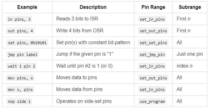
This table shows how PIO interprets the terms pin and pins in different instructions, along with their associated contexts and configurations.
Example: Distance program for the range finder
Here’s a PIO program for measuring the distance to an object using Trigger and Echo pins. The key features of this program are:
- Continuous Operation: The range finder runs in a loop as fast as possible.
- Maximum Range Limit: Measurements are capped at a given distance, with a return value of
4,294,967,295if no object is detected. - Filtered Outputs: Only measurements that differ from their immediate predecessor are sent, reducing the output rate.
Glance over the program and notice that although it is working with two pins — Trigger and Echo — throughout the program we only see pin and pins.
.program distance

; X is the last value sent. Initialize it to
; u32::MAX which means 'echo timeout'
; (Set X to u32::MAX by subtracting 1 from 0)
   set x, 0
subtraction_trick:
   jmp x-- subtraction_trick

; Read the max echo wait into OSR
   pull                         ; same as pull block

; Main loop
.wrap_target
   ; Generate 10μs trigger pulse (4 cycles at 343_000Hz)
   set pins, 0b1 [3]       ; Set trigger pin to high, add delay of 3
   set pins, 0b0           ; Set trigger pin to low voltage

   ; When the trigger goes high, start counting down until it goes low
   wait 1 pin 0            ; Wait for echo pin to be high voltage
   mov y, osr              ; Load max echo wait into Y

measure_echo_loop:
   jmp pin echo_active     ; if echo voltage is high continue count down
   jmp measurement_complete ; if echo voltage is low, measurement is complete
echo_active:
   jmp y-- measure_echo_loop ; Continue counting down unless timeout

; Y tells where the echo countdown stopped. It
; will be u32::MAX if the echo timed out.
measurement_complete:
   jmp x!=y send_result    ; if measurement is different, then sent it.
   jmp cooldown            ; If measurement is the same, don't send.

send_result:
   mov isr, y              ; Store measurement in ISR
   push                    ; Output ISR
   mov x, y               ; Save the measurement in X

; Cool down period before next measurement
cooldown:
   wait 0 pin 0           ; Wait for echo pin to be low
.wrap                      ; Restart the measurement loop
Configuring Pins
To ensure the PIO program behaves as intended:
set pins, 0b1should control the Trigger pin.wait 1 pin 0should monitor the Echo pin.jmp pin echo_activeshould also monitor the Echo pin.
Here’s how you can configure this in Rust (followed by an explanation):
let mut distance_state_machine = pio1.sm0;
let trigger_pio = pio1.common.make_pio_pin(hardware.trigger);
let echo_pio = pio1.common.make_pio_pin(hardware.echo);
distance_state_machine.set_pin_dirs(Direction::Out, &[&trigger_pio]);
distance_state_machine.set_pin_dirs(Direction::In, &[&echo_pio]);
distance_state_machine.set_config(&{
   let mut config = Config::default();
   config.set_set_pins(&[&trigger_pio]); // For set instruction
   config.set_in_pins(&[&echo_pio]); // For wait instruction
   config.set_jmp_pin(&echo_pio); // For jmp instruction
   let program_with_defines = pio_file!("examples/distance.pio");
   let program = pio1.common.load_program(&program_with_defines.program);
   config.use_program(&program, &[]); // No side-set pins
   config
});
The keys here are the set_set_pins, set_in_pins, and set_jmp_pin methods on the Config struct.
set_in_pins: Specifies the pins for input operations, such as wait(1, pin, …). The “in” pins must be consecutive.set_set_pins: Configures the pin for set operations, like set(pins, 1). The “set” pins must also be consecutive.set_jmp_pin: Defines the single pin used in conditional jumps, such asjmp(pin, ...).
As described in the table, other optional inputs include:
set_out_pins: Sets the consecutive pins for output operations, such as out(pins, …).use_program: Sets a) the loaded program and b) consecutive pins for sideset operations. Sideset operations allow simultaneous pin toggling during other instructions.
Configuring Multiple Pins
Although not required for this program, you can configure a range of pins in PIO by providing a slice of consecutive pins. For example, suppose we had two ultrasonic range finders:
let trigger_a_pio = pio1.common.make_pio_pin(hardware.trigger_a);
let trigger_b_pio = pio1.common.make_pio_pin(hardware.trigger_b);
config.set_set_pins(&[&trigger_a_pio, &trigger_b_pio]);
A single instruction can then control both pins:
set pins, 0b11 [3]  # Sets both trigger pins (17, 18) high, adds delay
set pins, 0b00      # Sets both trigger pins low
This approach lets you efficiently apply bit patterns to multiple pins simultaneously, streamlining control for applications involving multiple outputs.
Aside: The Word “Set” in Programming
In programming, the word “set” is notoriously overloaded with multiple meanings. In the context of PIO, “set” refers to something to which you can assign a value — such as a pin’s state. It does not mean a collection of things, as it often does in other programming contexts. When PIO refers to a collection, it usually uses the term “range” instead. This distinction is crucial for avoiding confusion as you work with PIO.
Lessons from Mrs. McCave
In Too Many Daves, Mrs. McCave lamented not giving her 23 Daves more distinct names. You can avoid her mistake by clearly documenting your pins with meaningful names — like Trigger and Echo — in your comments.
But if you think handling these pin ranges is tricky, debugging a PIO program adds an entirely new layer of challenge. In the next Wat, we’ll dive into the kludgy debugging methods available. Let’s see just how far we can push them.
I like to debug with interactive breakpoints in VS Code. I also do print debugging, where you insert temporary info statements to see what the code is doing and the values of variables. Using the Raspberry Pi Debug Probe and probe-rs, I can do both of these with regular Rust code on the Pico.
With PIO programming, however, I can do neither.
The fallback is push-to-print debugging. In PIO, you temporarily output integer values of interest. Then, in Rust, you use info! to print those values for inspection.
For example, in the following PIO program, we temporarily add instructions to push the value of x for debugging. We also include set and out to push a constant value, such as 7, which must be between 0 and 31 inclusive.
.program distance

; X is the last value sent. Initialize it to
; u32::MAX which means 'echo timeout'
; (Set X to u32::MAX by subtracting 1 from 0)
   set x, 0
subtraction_trick:
   jmp x-- subtraction_trick

; DEBUG: See the value of x
   mov isr, x
   push

; Read the max echo wait into OSR
   pull                         ; same as pull block

; DEBUG: Send constant value
   set y, 7           ; Push '7' so that we know we've reached this point
   mov isr, y
   push
; ...
Back in Rust, you can read and print these values to help understand what’s happening in the PIO code (full code and project):
  // ...
   distance_state_machine.set_enable(true);
   distance_state_machine.tx().wait_push(MAX_LOOPS).await;
   loop {
       let end_loops = distance_state_machine.rx().wait_pull().await;
       info!("end_loops: {}", end_loops);
   }
  // ...
Outputs:
INFO  Hello, debug!
└─ distance_debug::inner_main::{async_fn#0} @ examplesdistance_debug.rs:27
INFO  end_loops: 4294967295
└─ distance_debug::inner_main::{async_fn#0} @ examplesdistance_debug.rs:57
INFO  end_loops: 7
└─ distance_debug::inner_main::{async_fn#0} @ examplesdistance_debug.rs:57
When push-to-print debugging isn’t enough, you can turn to hardware tools. I bought my first oscilloscope (a FNIRSI DSO152, for $37). With it, I was able to confirm the Echo signal was working. The Trigger signal, however, was too fast for this inexpensive oscilloscope to capture clearly.
Using these methods — especially push-to-print debugging — you can trace the flow of your PIO program, even without a traditional debugger.
Aside: In C/C++ (and potentially Rust), you can get closer to a full debugging experience for PIO, for example, by using the piodebug project.
That concludes the nine Wats, but let’s bring everything together in a bonus Wat.
Now that all the components are ready, it’s time to combine them into a working theremin-like musical instrument. We need a Rust monitor program. This program starts both PIO state machines — one for measuring distance and the other for generating tones. It then waits for a new distance measurement, maps that distance to a tone, and sends the corresponding tone frequency to the tone-playing state machine. If the distance is out of range, it stops the tone.
Rust’s Place: At the heart of this system is a function that maps distances (from 0 to 50 cm) to tones (approximately B2 to F5). This function is simple to write in Rust, leveraging Rust’s floating-point math and exponential operations. Implementing this in PIO would be virtually impossible due to its limited instruction set and lack of floating-point support.
Here’s the core monitor program to run the theremin (full file and project):
sound_state_machine.set_enable(true);
distance_state_machine.set_enable(true);
distance_state_machine.tx().wait_push(MAX_LOOPS).await;
loop {
   let end_loops = distance_state_machine.rx().wait_pull().await;
   match loop_difference_to_distance_cm(end_loops) {
       None => {
           info!("Distance: out of range");
           sound_state_machine.tx().wait_push(0).await;
       }
       Some(distance_cm) => {
           let tone_frequency = distance_to_tone_frequency(distance_cm);
           let half_period = sound_state_machine_frequency / tone_frequency as u32 / 2;
           info!("Distance: {} cm, tone: {} Hz", distance_cm, tone_frequency);
           sound_state_machine.tx().push(half_period); // non-blocking push
           Timer::after(Duration::from_millis(50)).await;
       }
   }
}
Using two PIO state machines alongside a Rust monitor program lets you literally run three programs at once. This setup is convenient on its own and is essential when strict timing or very high-frequency I/O operations are required.
Aside: Alternatively, Rust Embassy’s async tasks let you implement cooperative multitasking directly on a single main processor. You code in Rust rather than a mixture of Rust and PIO. Although Embassy tasks don’t literally run in parallel, they switch quickly enough to handle applications like a theremin. Here’s a snippet from theremin_no_pio.rs showing a similar core loop:
loop {
       match distance.measure().await {
           None => {
               info!("Distance: out of range");
               sound.rest().await;
           }
           Some(distance_cm) => {
               let tone_frequency = distance_to_tone_frequency(distance_cm);
               info!("Distance: {} cm, tone: {} Hz", distance_cm, tone_frequency);
               sound.play(tone_frequency).await;
               Timer::after(Duration::from_millis(50)).await;
           }
       }
   }
See our recent article on Rust Embassy programming for more details.
Now that we’ve assembled all the components, let’s watch the video again of me “playing” the musical instrument. On the monitor screen, you can see the debugging prints displaying the distance measurements and the corresponding tones. This visual connection highlights how the system responds in real time.
Conclusion
PIO programming on the Raspberry Pi Pico is a captivating blend of simplicity and complexity, offering unparalleled hardware control while demanding a shift in mindset for developers accustomed to higher-level programming. Through the nine Wats we’ve explored, PIO has both surprised us with its limitations and impressed us with its raw efficiency.
While we’ve covered significant ground — managing state machines, pin assignments, timing intricacies, and debugging — there’s still much more you can learn as needed: DMA, IRQ, side-set pins, differences between PIO on the Pico 1 and Pico 2, autopush and autopull, FIFO join, and more.
Recommended Resources
At its core, PIO’s quirks reflect a design philosophy that prioritizes low-level hardware control with minimal overhead. By embracing these characteristics, PIO will not only meet your project’s demands but also open doors to new possibilities in embedded systems programming.
Please follow Carl on Towards Data Science and on @carlkadie.bsky.social. I write on scientific programming in Rust and Python, machine learning, and statistics. I tend to write about one article per month.