You’ve probably used the normal distribution one or two times too many. We all have — It’s a true workhorse. But sometimes, we run into problems. For instance, when predicting or forecasting values, simulating data given a particular data-generating process, or when we try to visualise model output and explain them intuitively to non-technical stakeholders. Suddenly, things don’t make much sense: can a user really have made -8 clicks on the banner? Or even 4.3 clicks? Both are examples of how count data doesn’t behave.
I’ve found that better encapsulating the data generating process into my modelling has been key to having sensible model output. Using the Poisson distribution when it was appropriate has not only helped me convey more meaningful insights to stakeholders, but it has also enabled me to produce more accurate error estimates, better Inference, and sound decision-making.
In this post, my aim is to help you get a deep intuitive feel for the Poisson distribution by walking through example applications, and taking a dive into the foundations — the maths. I hope you learn not just how it works, but also why it works, and when to apply the distribution.
If you know of a resource that has helped you grasp the concepts in this blog particularly well, you’re invited to share it in the comments!
Outline
- Examples and use cases: Let’s walk through some use cases and sharpen the intuition I just mentioned. Along the way, the relevance of the Poisson Distribution will become clear.
- The foundations: Next, let’s break down the equation into its individual components. By studying each part, we’ll uncover why the distribution works the way it does.
- The assumptions: Equipped with some formality, it will be easier to understand the assumptions that power the distribution, and at the same time set the boundaries for when it works, and when not.
- When real life deviates from the model: Finally, let’s explore the special links that the Poisson distribution has with the Negative Binomial distribution. Understanding these relationships can deepen our understanding, and provide alternatives when the Poisson distribution is not suited for the job.
Example in an online marketplace
I chose to deep dive into the Poisson distribution because it frequently appears in my day-to-day work. Online marketplaces rely on binary user choices from two sides: a seller deciding to list an item and a buyer deciding to make a purchase. These micro-behaviours drive supply and demand, both in the short and long term. A marketplace is born.
Binary choices aggregate into counts — the sum of many such decisions as they occur. Attach a timeframe to this counting process, and you’ll start seeing Poisson distributions everywhere. Let’s explore a concrete example next.
Consider a seller on a platform. In a given month, the seller may or may not list an item for sale (a binary choice). We would only know if she did because then we’d have a measurable count of the event. Nothing stops her from listing another item in the same month. If she does, we count those events. The total could be zero for an inactive seller or, say, 120 for a highly engaged seller.
Over several months, we would observe a varying number of listed items by this seller — sometimes fewer, sometimes more — hovering around an average monthly listing rate. That is essentially a Poisson process. When we get to the assumptions section, you’ll see what we had to assume away to make this example work.
Other examples
Other phenomena that can be modelled with a Poisson distribution include:
- Sports analytics: The number of goals scored in a match between two teams.
- Queuing: Customers arriving at a help desk or customer support calls.
- Insurance: The number of claims made within a given period.
Each of these examples warrants further inspection, but for the remainder of this post, we’ll use the marketplace example to illustrate the inner workings of the distribution.
The mathy bit
… or foundations.
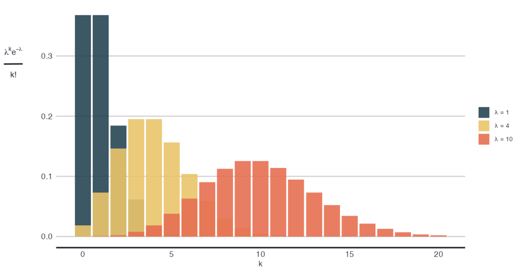
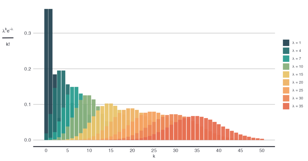
I find opening up the probability mass function (PMF) of distributions helpful to understanding why things work as they do. The PMF of the Poisson distribution goes like:

Where λ is the rate parameter, and 𝑘 is the manifested count of the random variable (𝑘 = 0, 1, 2, 3, … events). Very neat and compact.
Contextualising λ and k: the marketplace example
In the context of our earlier example — a seller listing items on our platform — λ represents the seller’s average monthly listings. As the expected monthly value for this seller, λ orchestrates the number of items she would list in a month. Note that λ is a Greek letter, so read: λ is a parameter that we can estimate from data. On the other hand, 𝑘 does not hold any information about the seller’s idiosyncratic behaviour. It’s the target value we set for the number of events that may happen to learn about its probability.
The dual role of λ as the mean and variance
When I said that λ orchestrates the number of monthly listings for the seller, I meant it quite literally. Namely, λ is both the expected value and variance of the distribution, indifferently, for all values of λ. This means that the mean-to-variance ratio (index of dispersion) is always 1.
To put this into perspective, the normal distribution requires two parameters — 𝜇 and 𝜎², the average and variance respectively — to fully describe it. The Poisson distribution achieves the same with just one.
Having to estimate only one parameter can be beneficial for parametric inference. Specifically, by reducing the variance of the model and increasing the statistical power. On the other hand, it can be too limiting of an assumption. Alternatives like the Negative Binomial distribution can alleviate this limitation. We’ll explore that later.
Breaking down the probability mass function
Now that we know the smallest building blocks, let’s zoom out one step: what is λᵏ, 𝑒^⁻λ, and 𝑘!, and more importantly, what is each of these components’ function in the whole?
- λᵏ is a weight that expresses how likely it is for 𝑘 events to happen, given that the expectation is λ. Note that “likely” here does not mean a probability, yet. It’s merely a signal strength.
- 𝑘! is a combinatorial correction so that we can say that the order of the events is irrelevant. The events are interchangeable.
- 𝑒^⁻λ normalises the integral of the PMF function to sum up to 1. It’s called the partition function of exponential-family distributions.
In more detail, λᵏ relates the observed value 𝑘 to the expected value of the random variable, λ. Intuitively, more probability mass lies around the expected value. Hence, if the observed value lies close to the expectation, the probability of occurring is larger than the probability of an observation far removed from the expectation. Before we can cross-check our intuition with the numerical behaviour of λᵏ, we need to consider what 𝑘! does.
Interchangeable events
Had we cared about the order of events, then each unique event could be ordered in 𝑘! ways. But because we don’t, and we deem each event interchangeable, we “divide out” 𝑘! from λᵏ to correct for the overcounting.
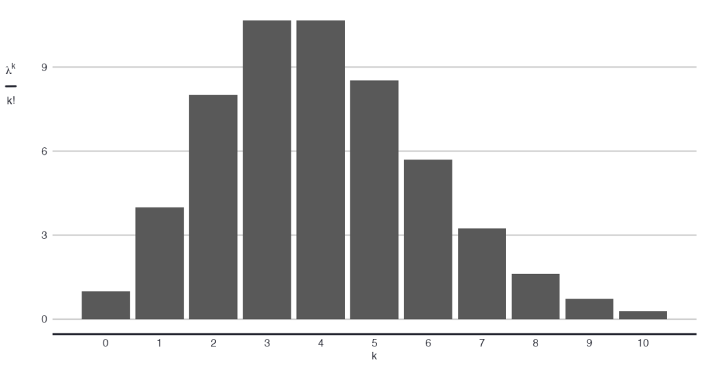
Since λᵏ is an exponential term, the output will always be larger as 𝑘 grows, holding λ constant. That is the opposite of our intuition that there is maximum probability when λ = 𝑘, as the output is larger when 𝑘 = λ + 1. But now that we know about the interchangeable events assumption — and the overcounting issue — we know that we have to factor in 𝑘! like so: λᵏ 𝑒^⁻λ / 𝑘!, to see the behaviour we expect.
Now let’s check the intuition of the relationship between λ and 𝑘 through λᵏ, corrected for 𝑘!. For the same λ, say λ = 4, we should see λᵏ 𝑒^⁻λ / 𝑘! to be smaller for values of 𝑘 that are far removed from 4, compared to values of 𝑘 that lie close to 4. Like so: inline code: 4²/2 = 8 is smaller than 4⁴/24 = 10.7. This is consistent with the intuition of a higher likelihood of 𝑘 when it’s near the expectation. The image below shows this relationship more generally, where you see that the output is larger as 𝑘 approaches λ.
The assumptions
First, let’s get one thing off the table: the difference between a Poisson process, and the Poisson distribution. The process is a stochastic continuous-time model of points happening in given interval: 1D, a line; 2D, an area, or higher dimensions. We, data scientists, most often deal with the one-dimensional case, where the “line” is time, and the points are the events of interest — I dare to say.
These are the assumptions of the Poisson process:
- The occurrence of one event does not affect the probability of a second event. Think of our seller going on to list another item tomorrow indifferently of having done so already today, or the one from five days ago for that matter. The point here is that there is no memory between events.
- The average rate at which events occur, is independent of any occurrence. In other words, no event that happened (or will happen) alters λ, which remains constant throughout the observed timeframe. In our seller example, this means that listing an item today does not increase or decrease the seller’s motivation or likelihood of listing another item tomorrow.
- Two events cannot occur at exactly the same instant. If we were to zoom at an infinite granular level on the timescale, no two listings could have been placed simultaneously; always sequentially.
From these assumptions — no memory, constant rate, events happening alone — it follows that 1) any interval’s number of events is Poisson-distributed with parameter λₜ and 2) that disjoint intervals are independent — two key properties of a Poisson process.
A Note on the distribution:
The distribution simply describes probabilities for various numbers of counts in an interval. Strictly speaking, one can use the distribution pragmatically whenever the data is nonnegative, can be unbounded on the right, has mean λ, and reasonably models the data. It would be just convenient if the underlying process is a Poisson one, and actually justifies using the distribution.
The marketplace example: Implications
So, can we justify using the Poisson distribution for our marketplace example? Let’s open up the assumptions of a Poisson process and take the test.
Constant λ
- Why it may fail: The seller has patterned online activity; holidays; promotions; listings are seasonal goods.
- Consequence: λ is not constant, leading to overdispersion (mean-to-variance ratio is larger than 1, or to temporal patterns.
Independence and memorylessness
- Why it may fail: The propensity to list again is higher after a successful listing, or conversely, listing once depletes the stock and intervenes with the propensity of listing again.
- Consequence: Two events are no longer independent, as the occurrence of one informs the occurrence of the other.
Simultaneous events
- Why it may fail: Batch-listing, a new feature, was introduced to help the sellers.
- Consequence: Multiple listings would come online at the same time, clumped together, and they would be counted simultaneously.
Balancing rigour and pragmatism
As Data Scientists on the job, we may feel trapped between rigour and pragmatism. The three steps below should give you a sound foundation to decide on which side to err, when the Poisson distribution falls short:
- Pinpoint your goal: is it inference, simulation or prediction, and is it about high-stakes output? List the worst thing that can happen, and the cost of it for the business.
- Identify the problem and solution: why does the Poisson distribution not fit, and what can you do about it? list 2-3 solutions, including changing nothing.
- Balance gains and costs: Will your workaround improve things, or make it worse? and at what cost: interpretability, new assumptions introduced and resources used. Does it help you in achieving your goal?
That said, here are some counters I use when needed.
When real life deviates from your model
Everything described so far pertains to the standard, or homogenous, Poisson process. But what if reality begs for something different?
In the next section, we’ll cover two extensions of the Poisson distribution when the constant λ assumption does not hold. These are not mutually exclusive, but neither they are the same:
- Time-varying λ: a single seller whose listing rate ramps up before holidays and slows down afterward
- Mixed Poisson distribution: multiple sellers listing items, each with their own λ can be seen as a mixture of various Poisson processes
Time-varying λ
The first extension allows λ to have its own value for each time t. The PMF then becomes

Where the number of events 𝐾(𝑇) in an interval 𝑇 follows the Poisson distribution with a rate no longer equal to a fixed λ, but one equal to:

More intuitively, integrating over the interval 𝑡 to 𝑡 + 𝑖 gives us a single number: the expected value of events over that interval. The integral will vary by each arbitrary interval, and that’s what makes λ change over time. To understand how that integration works, it was helpful for me to think of it like this: if the interval 𝑡 to 𝑡₁ integrates to 3, and 𝑡₁ to 𝑡₂ integrates to 5, then the interval 𝑡 to 𝑡₂ integrates to 8 = 3 + 5. That’s the two expectations summed up, and now the expectation of the entire interval.
Practical implication
One may want to modeling the expected value of the Poisson distribution as a function of time. For instance, to model an overall change in trend, or seasonality. In generative model notation:

Time may be a continuous variable, or an arbitrary function of it.
Process-varying λ: Mixed Poisson distribution
But then there’s a gotcha. Remember when I said that λ has a dual role as the mean and variance? That still applies here. Looking at the “relaxed” PMF*, the only thing that changes is that λ can vary freely with time. But it’s still the one and only λ that orchestrates both the expected value and the dispersion of the PMF*. More precisely, 𝔼[𝑋] = Var(𝑋) still holds.
There are various reasons for this constraint not to hold in reality. Model misspecification, event interdependence and unaccounted for heterogeneity could be the issues at hand. I’d like to focus on the latter case, as it justifies the Negative Binomial distribution — one of the topics I promised to open up.
Heterogeneity and overdispersion
Imagine we are not dealing with one seller, but with 10 of them listing at different intensity levels, λᵢ, where 𝑖 = 1, 2, 3, …, 10 sellers. Then, essentially, we have 10 Poisson processes going on. If we unify the processes and estimate the grand λ, we simplify the mixture away. Meaning, we get a correct estimate of all sellers on average, but the resulting grand λ is naive and does not know about the original spread of λᵢ. It still assumes that the variance and mean are equal, as per the axioms of the distribution. This will lead to overdispersion and, in turn, to underestimated errors. Ultimately, it inflates the false positive rate and drives poor decision-making. We need a way to embrace the heterogeneity amongst sellers’ λᵢ.
Negative binomial: Extending the Poisson distribution
Among the few ways one can look at the Negative Binomial distribution, one way is to see it as a compound Poisson process — 10 sellers, sounds familiar yet? That means multiple independent Poisson processes are summed up to a single one. Mathematically, first we draw λ from a Gamma distribution: λ ~ Γ(r, θ), then we draw the count 𝑋 | λ ~ Poisson(λ).
In one image, it is as if we would sample from plenty Poisson distributions, corresponding to each seller.
The more exposing alias of the Negative binomial distribution is Gamma-Poisson mixture distribution, and now we know why: the dictating λ comes from a continuous mixture. That’s what we needed to explain the heterogeneity amongst sellers.
Let’s simulate this scenario to gain more intuition.
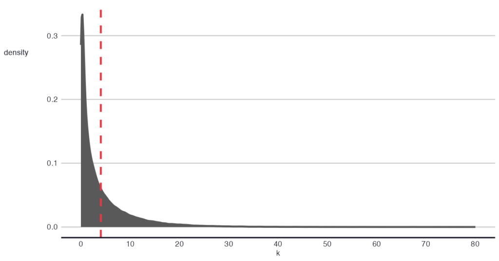
First, we draw λᵢ from a Gamma distribution: λᵢ ~ Γ(r, θ). Intuitively, the Gamma distribution tells us about the variety in the intensity — listing rate — amongst the sellers.
On a practical note, one can instill their assumptions about the degree of heterogeneity in this step of the model: how different are sellers? By varying the levels of heterogeneity, one can observe the impact on the final Poisson-like distribution. Doing this type of checks (i.e., posterior predictive check), is common in Bayesian modeling, where the assumptions are set explicitly.
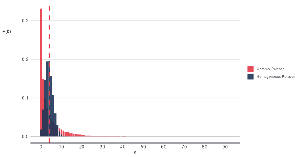
In the second step, we plug the obtained λ into the Poisson distribution: 𝑋 | λ ~ Poisson(λ), and obtain a Poisson-like distribution that represents the summed subprocesses. Notably, this unified process has a larger dispersion than expected from a homogeneous Poisson distribution, but it is in line with the Gamma mixture of λ.
Heterogeneous λ and inference
A practical consequence of introducing flexibility into your assumed distribution is that inference becomes more challenging. More parameters (i.e., the Gamma parameters) need to be estimated. Parameters act as flexible explainers of the data, tending to overfit and explain away variance in your variable. The more parameters you have, the better the explanation may seem, but the model also becomes more susceptible to noise in the data. Higher variance reduces the power to identify a difference in means, if one exists, because — well — it gets lost in the variance.
Countering the loss of power
- Confirm whether you indeed need to extend the standard Poisson distribution. If not, simplify to the simplest, most fit model. A quick check on overdispersion may suffice for this.
- Pin down the estimates of the Gamma mixture distribution parameters using regularising, informative priors (think: Bayes).
During my research process for writing this blog, I learned a great deal about the connective tissue underlying all of this: how the binomial distribution plays a fundamental role in the processes we’ve discussed. And while I’d love to ramble on about this, I’ll save it for another post, perhaps. In the meantime, feel free to share your understanding in the comments section below 👍.
Conclusion
The Poisson distribution is a simple distribution that can be highly suitable for modelling count data. However, when the assumptions do not hold, one can extend the distribution by allowing the rate parameter to vary as a function of time or other factors, or by assuming subprocesses that collectively make up the count data. This added flexibility can address the limitations, but it comes at a cost: increased flexibility in your modelling raises the variance and, consequently, undermines the statistical power of your model.
If your end goal is inference, you may want to think twice and consider exploring simpler models for the data. Alternatively, switch to the Bayesian paradigm and leverage its built-in solution to regularise estimates: informative priors.
I hope this has given you what you came for — a better intuition about the Poisson distribution. I’d love to hear your thoughts about this in the comments!
Unless otherwise noted, all images are by the author.
Originally published at https://aalvarezperez.github.io on January 5, 2025.