Your Gateway to Power, Energy, Datacenters, Bitcoin and AI

Dive into the latest industry updates, our exclusive Paperboy Newsletter, and curated insights designed to keep you informed. Stay ahead with minimal time spent.

Discover What Matters Most to You

Explore ONMINE’s curated content, from our Paperboy Newsletter to industry-specific insights tailored for energy, Bitcoin mining, and AI professionals.

AI

Lorem Ipsum is simply dummy text of the printing and typesetting industry.

Bitcoin:

Lorem Ipsum is simply dummy text of the printing and typesetting industry.

Datacenter:

Lorem Ipsum is simply dummy text of the printing and typesetting industry.

Energy:

Lorem Ipsum is simply dummy text of the printing and typesetting industry.

Shape
Discover What Matter Most to You

Featured Articles

Custom Training Pipeline for Object Detection Models

What if you want to write the whole object detection training pipeline from scratch, so you can understand each step and be able to customize it? That’s what I set out to do. I examined several well-known object detection pipelines and designed one that best suits my needs and tasks. Thanks to Ultralytics, YOLOx, DAMO-YOLO, RT-DETR and D-FINE repos, I leveraged them to gain deeper understanding into various design details. I ended up implementing SoTA real-time object detection model D-FINE in my custom pipeline.

Plan

Dataset, Augmentations and transforms:

Mosaic (with affine transforms)

Mixup and Cutout

Other augmentations with bounding boxes

Letterbox vs simple resize

Training:

Optimizer

Scheduler

EMA

Batch accumulation

AMP

Grad clipping

Logging

Metrics:

mAPs from TorchMetrics / cocotools

How to compute Precision, Recall, IoU?

Pick a suitable solution for your case

Experiments

Attention to data preprocessing

Where to start

Dataset

Dataset processing is the first thing you usually start working on. With object detection, you need to load your image and annotations. Annotations are often stored in COCO format as a json file or YOLO format, with txt file for each image. Let’s take a look at the YOLO format: Each line is structured as: class_id, x_center, y_center, width, height, where bbox values are normalized between 0 and 1.

When you have your images and txt files, you can write your dataset class, nothing tricky here. Load everything, transform (augmentations included) and return during training. I prefer splitting the data by creating a CSV file for each split and then reading it in the Dataloader class rather than physically moving files into train/val/test folders. This is an example of a customization that helped my use case.

Augmentations

Firstly, when augmenting images for object detection, it’s crucial to apply the same transformations to the bounding boxes. To comfortably do that I use Albumentations lib. For example:

    def _init_augs(self, cfg) – > None:
        if self.keep_ratio:
            resize = [
                A.LongestMaxSize(max_size=max(self.target_h, self.target_w)),
                A.PadIfNeeded(
                    min_height=self.target_h,
                    min_width=self.target_w,
                    border_mode=cv2.BORDER_CONSTANT,
                    fill=(114, 114, 114),
                ),
            ]

        else:
            resize = [A.Resize(self.target_h, self.target_w)]
        norm = [
            A.Normalize(mean=self.norm[0], std=self.norm[1]),
            ToTensorV2(),
        ]

        if self.mode == “train”:
            augs = [
                A.RandomBrightnessContrast(p=cfg.train.augs.brightness),
                A.RandomGamma(p=cfg.train.augs.gamma),
                A.Blur(p=cfg.train.augs.blur),
                A.GaussNoise(p=cfg.train.augs.noise, std_range=(0.1, 0.2)),
                A.ToGray(p=cfg.train.augs.to_gray),
                A.Affine(
                    rotate=[90, 90],
                    p=cfg.train.augs.rotate_90,
                    fit_output=True,
                ),
                A.HorizontalFlip(p=cfg.train.augs.left_right_flip),
                A.VerticalFlip(p=cfg.train.augs.up_down_flip),
            ]

            self.transform = A.Compose(
                augs + resize + norm,
                bbox_params=A.BboxParams(format=”pascal_voc”, label_fields=[“class_labels”]),
            )

        elif self.mode in [“val”, “test”, “bench”]:
            self.mosaic_prob = 0
            self.transform = A.Compose(
                resize + norm,
                bbox_params=A.BboxParams(format=”pascal_voc”, label_fields=[“class_labels”]),
            )

Secondly, there are a lot of interesting and not trivial augmentations:

Mosaic. The idea is simple, let’s take several images (for example 4), and stack them together in a grid (2×2). Then let’s do some affine transforms and feed it to the model.

MixUp. Originally used in image classification (it’s surprising that it works). Idea – let’s take two images, put them onto each other with some percent of transparency. In classification models it usually means that if one image is 20% transparent and the second is 80%, then the model should predict 80% for class 1 and 20% for class 2. In object detection we just get more objects into 1 image.

Cutout. Cutout involves removing parts of the image (by replacing them with black pixels) to help the model learn more robust features.

I see mosaic often applied with Probability 1.0 of the first ~90% of epochs. Then, it’s usually turned off, and lighter augmentations are used. The same idea applies to mixup, but I see it being used a lot less (for the most popular detection framework, Ultralytics, it’s turned off by default. For another one, I see P=0.15). Cutout seems to be used less frequently.

You can read more about those augmentations in these two articles: 1, 2.

Results from just turning on mosaic are pretty good (darker one without mosaic got mAP 0.89 vs 0.92 with, tested on a real dataset) 

Author’s metrics on a custom dataset, logged in Wandb

Letterbox or simple resize?

During training, you usually resize the input image to a square. Models often use 640×640 and benchmark on COCO dataset. And there are two main ways how you get there:

Simple resize to a target size.

Letterbox: Resize the longest side to the target size (e.g., 640), preserving the aspect ratio, and pad the shorter side to reach the target dimensions.

Sample from VisDrone dataset with ground truth bounding boxes, preprocessed with a simple resize function

Sample from VisDrone dataset with ground truth bounding boxes, preprocessed with a letterbox

Both approaches have advantages and disadvantages. Let’s discuss them first, and then I will share the results of numerous experiments I ran comparing these approaches.

Simple resize:

Compute goes to the whole image, with no useless padding.

“Dynamic” aspect ratio may act as a form of regularization.

Inference preprocessing perfectly matches training preprocessing (augmentations excluded).

Kills real geometry. Resize distortion could affect the spatial relationships in the image. Although it might be a human bias to think that a fixed aspect ratio is important.

Letterbox:

Preserves real aspect ratio.

During inference, you can cut padding and run not on the square image if you don’t lose accuracy (some models can degrade).

Can train on a bigger image size, then inference with cut padding to get the same inference latency as with simple resize. For example 640×640 vs 832×480. The second one will preserve the aspect ratios and objects will appear +- the same size.

Part of the compute is wasted on gray padding.

Objects get smaller.

How to test it and decide which one to use? 

Train from scratch with parameters:

Simple resize, 640×640

Keep aspect ratio, max side 640, and add padding (as a baseline)

Keep aspect ratio, larger image size (for example max side 832), and add padding Then inference 3 models. When the aspect ratio is preserved – cut padding during the inference. Compare latency and metrics.

Example of the same image from above with cut padding (640 × 384): 

Sample from VisDrone dataset

Here is what happens when you preserve ratio and inference by cutting gray padding:

params                  |  F1 score  | latency (ms). |
————————-+————-+—————–|
ratio kept, 832        |    0.633    |        33.5      |
no ratio, 640×640   |    0.617    |        33.4      |

As shown, training with preserved aspect ratio at a larger size (832) achieved a higher F1 score (0.633) compared to a simple 640×640 resize (F1 score of 0.617), while the latency remained similar. Note that some models may degrade if the padding is removed during inference, which kills the whole purpose of this trick and probably the letterbox too.

What does this mean: 

Training from scratch:

With the same image size, simple resize gets better accuracy than letterbox.

For letterbox, If you cut padding during the inference and your model doesn’t lose accuracy – you can train and inference with a bigger image size to match the latency, and get a little bit higher metrics (as in the example above). 

Training with pre-trained weights initialized:

If you finetune – use the same tactic as the pre-trained model did, it should give you the best results if the datasets are not too different.

For D-FINE I see lower metrics when cutting padding during inference. Also the model was pre-trained on a simple resize. For YOLO, a letterbox is typically a good choice.

Training

Every ML engineer should know how to implement a training loop. Although PyTorch does much of the heavy lifting, you might still feel overwhelmed by the number of design choices available. Here are some key components to consider:

Optimizer – start with Adam/AdamW/SGD.

Scheduler – fixed LR can be ok for Adams, but take a look at StepLR, CosineAnnealingLR or OneCycleLR.

EMA. This is a nice technique that makes training smoother and sometimes achieves higher metrics. After each batch, you update a secondary model (often called the EMA model)  by computing an exponential moving average of the primary model’s weights.

Batch accumulation is nice when your vRAM is very limited. Training a transformer-based object detection model means that in some cases even in a middle-sized model you only can fit 4 images into the vRAM. By accumulating gradients over several batches before performing an optimizer step, you effectively simulate a larger batch size without exceeding your memory constraints. Another use case is when you have a lot of negatives (images without target objects) in your dataset and a small batch size, you can encounter unstable training. Batch accumulation can also help here.

AMP uses half precision automatically where applicable. It reduces vRAM usage and makes training faster (if you have a GPU that supports it). I see 40% less vRAM usage and at least a 15% training speed increase.

Grad clipping. Often, when you use AMP, training can become less stable. This can also happen with higher LRs. When your gradients are too big, training will fail. Gradient clipping will make sure gradients are never bigger than a certain value.

Logging. Try Hydra for configs and something like Weights and Biases or Clear ML for experiment tracking. Also, log everything locally. Save your best weights, and metrics, so after numerous experiments, you can always find all the info on the model you need.

    def train(self) – > None:
        best_metric = 0
        cur_iter = 0
        ema_iter = 0
        one_epoch_time = None

        def optimizer_step(step_scheduler: bool):
            “””
            Clip grads, optimizer step, scheduler step, zero grad, EMA model update
            “””
            nonlocal ema_iter
            if self.amp_enabled:
                if self.clip_max_norm:
                    self.scaler.unscale_(self.optimizer)

torch.nn.utils.clip_grad_norm_(self.model.parameters(), self.clip_max_norm)
                self.scaler.step(self.optimizer)
                self.scaler.update()

            else:
                if self.clip_max_norm:

torch.nn.utils.clip_grad_norm_(self.model.parameters(), self.clip_max_norm)
                self.optimizer.step()

            if step_scheduler:
                self.scheduler.step()
            self.optimizer.zero_grad()

            if self.ema_model:
                ema_iter += 1
                self.ema_model.update(ema_iter, self.model)

        for epoch in range(1, self.epochs + 1):
            epoch_start_time = time.time()
            self.model.train()
            self.loss_fn.train()
            losses = []

            with tqdm(self.train_loader, unit=”batch”) as tepoch:
                for batch_idx, (inputs, targets, _) in enumerate(tepoch):
                    tepoch.set_description(f”Epoch {epoch}/{self.epochs}”)
                    if inputs is None:
                        continue
                    cur_iter += 1

                    inputs = inputs.to(self.device)
                    targets = [
                        {
                            k: (v.to(self.device) if (v is not None and hasattr(v, “to”)) else v)
                            for k, v in t.items()
                        }
                        for t in targets
                    ]

                    lr = self.optimizer.param_groups[0][“lr”]

                    if self.amp_enabled:
                        with autocast(self.device, cache_enabled=True):
                            output = self.model(inputs, targets=targets)
                        with autocast(self.device, enabled=False):
                            loss_dict = self.loss_fn(output, targets)
                        loss = sum(loss_dict.values()) / self.b_accum_steps
                        self.scaler.scale(loss).backward()

                    else:
                        output = self.model(inputs, targets=targets)
                        loss_dict = self.loss_fn(output, targets)
                        loss = sum(loss_dict.values()) / self.b_accum_steps
                        loss.backward()

                    if (batch_idx + 1) % self.b_accum_steps == 0:
                        optimizer_step(step_scheduler=True)

                    losses.append(loss.item())

                    tepoch.set_postfix(
                        loss=np.mean(losses) * self.b_accum_steps,
                        eta=calculate_remaining_time(
                            one_epoch_time,
                            epoch_start_time,
                            epoch,
                            self.epochs,
                            cur_iter,
                            len(self.train_loader),
                        ),
                        vram=f”{get_vram_usage()}%”,
                    )

            # Final update for any leftover gradients from an incomplete accumulation step
            if (batch_idx + 1) % self.b_accum_steps != 0:
                optimizer_step(step_scheduler=False)

            wandb.log({“lr”: lr, “epoch”: epoch})

            metrics = self.evaluate(
                val_loader=self.val_loader,
                conf_thresh=self.conf_thresh,
                iou_thresh=self.iou_thresh,
                path_to_save=None,
            )

            best_metric = self.save_model(metrics, best_metric)
            save_metrics(
                {}, metrics, np.mean(losses) * self.b_accum_steps, epoch, path_to_save=None
            )

            if (
                epoch >= self.epochs – self.no_mosaic_epochs
                and self.train_loader.dataset.mosaic_prob
            ):
                self.train_loader.dataset.close_mosaic()

            if epoch == self.ignore_background_epochs:
                self.train_loader.dataset.ignore_background = False
                logger.info(“Including background images”)

            one_epoch_time = time.time() – epoch_start_time

Metrics

For object detection everyone uses mAP, and it is already standardized how we measure those. Use pycocotools or faster-coco-eval or TorchMetrics for mAP. But mAP means that we check how good the model is overall, on all confidence levels. mAP0.5 means that IoU threshold is 0.5 (everything lower is considered as a wrong prediction). I personally don’t fully like this metric, as in production we always use 1 confidence threshold. So why not set the threshold and then compute metrics? That’s why I also always calculate confusion matrices, and based on that – Precision, Recall, F1-score, and IoU.

But logic also might be tricky. Here is what I use:

1 GT (ground truth) object = 1 predicted object, and it’s a TP if IoU > threshold. If there is no prediction for a GT object – it’s a FN. If there is no GT for a prediction – it’s a FP.

1 GT should be matched by a prediction only 1 time. If there are 2 predictions for 1 GT, then I calculate 1 TP and 1 FP.

Class ids should also match. If the model predicts class_0 but GT is class_1, it means FP += 1 and FN += 1.

During training, I select the best model based on the metrics that are relevant to the task. I typically consider the average of mAP50 and F1-score.

Model and loss

I haven’t discussed model architecture and loss function here. They usually go together, and you can choose any model you like and integrate it into your pipeline with everything from above. I did that with DAMO-YOLO and D-FINE, and the results were great.

Pick a suitable solution for your case

Many people use Ultralytics, however it has GPLv3, and you can’t use it in commercial projects unless your code is open source. So people often look into Apache 2 and MIT licensed models. Check out D-FINE, RT-DETR2 or some yolo models like Yolov9.

What if you want to customize something in the pipeline? When you build everything from scratch, you should have full control. Otherwise, try choosing a project with a smaller codebase, as a large one can make it difficult to isolate and modify individual components.

If you don’t need anything custom and your usage is allowed by the Ultralytics license – it’s a great repo to use, as it supports multiple tasks (classification, detection, instance segmentation, key points, oriented bounding boxes), models are efficient and achieve good scores. Reiterating ones more, you probably don’t need a custom training pipeline if you are not doing very specific things.

Experiments

Let me share some results I got with a custom training pipeline with the D-FINE model and compare it to the Ultralytics YOLO11 model on the VisDrone-DET2019 dataset.

Trained from scratch:

model                     |  mAP 0.50. |  F1-score | Latency (ms) |
———————————+————–+————–+——————|
YOLO11m TRT               |     0.417    |     0.568    |       15.6     |
YOLO11m TRT dynamic |    –    |     0.568   |       13.3     |
YOLO11m OV                |      –      |     0.568   |      122.4     |
D-FINEm TRT               |    0.457    |     0.622   |       16.6    |
D-FINEm OV                |    0.457    |     0.622    |       115.3    |

From COCO pre-trained:

model          |  mAP 0.50 |  F1-score  |
——————+————|————-|
YOLO11m     |     0.456     |    0.600   |
D-FINEm       |     0.506     |    0.649    |

Latency was measured on an RTX 3060 with TensorRT (TRT), static image size 640×640, including the time for cv2.imread. OpenVINO (OV) on i5 14000f (no iGPU). Dynamic means that during inference, gray padding is being cut for faster inference. It worked with the YOLO11 TensorRT version. More details about cutting gray padding above (Letterbox or simple resize section).

One disappointing result is the latency on intel N100 CPU with iGPU ($150 miniPC):

model            | Latency (ms) |
——————+————-|
YOLO11m      |       188    |
D-FINEm      |       272    |
D-FINEs         |       11     |

Author’s screenshot of iGPU usage from n100 machine during model inference

Here, traditional convolutional neural networks are noticeably faster, maybe because of optimizations in OpenVINO for GPUs.

Overall, I conducted over 30 experiments with different datasets (including real-world datasets), models, and parameters and I can say that D-FINE gets better metrics. And it makes sense, as on COCO, it is also higher than all YOLO models. 

D-FINE paper comparison to other object detection models

VisDrone experiments: 

Author’s metrics logged in WandB, D-FINE model

Author’s metrics logged in WandB, YOLO11 model

Example of D-FINE model predictions (green – GT, blue – pred): 

Sample from VisDrone dataset

Final results

Knowing all the details, let’s see a final comparison with the best settings for both models on i12400F and RTX 3060 with the VisDrone dataset:

model                             |   F1-score  | Latency (ms) |
———————————–+—————+——————-|
YOLO11m TRT dynamic   |      0.600    |        13.3     |
YOLO11m OV                   |      0.600    |       122.4      |
D-FINEs TRT                  |      0.629    |        12.3     |
D-FINEs OV                      |      0.629    |        57.4       |

As shown above, I was able to use a smaller D-FINE model and achieve both faster inference time and accuracy than YOLO11. Beating Ultralytics, the most widely used real-time object detection model, in both speed and accuracy, is quite an accomplishment, isn’t it? The same pattern is observed across several other real-world datasets.

I also tried out YOLOv12, which came out while I was writing this article. It performed similarly to YOLO11 and even achieved slightly lower metrics (mAP 0.456 vs 0.452). It appears that YOLO models have been hitting the wall for the last couple of years. D-FINE was a great update for object detection models.

Finally, let’s see visually the difference between YOLO11m and D-FINEs. YOLO11m, conf 0.25, nms iou 0.5, latency 13.3ms: 

Sample from VisDrone dataset

D-FINEs, conf 0.5, no nms, latency 12.3ms: 

Sample from VisDrone dataset

Both Precision and Recall are higher with the D-FINE model. And it’s also faster. Here is also “m” version of D-FINE: 

Sample from VisDrone dataset

Isn’t it crazy that even that one car on the left was detected?

Attention to data preprocessing

This part can go a little bit outside the scope of the article, but I want to at least quickly mention it, as some parts can be automated and used in the pipeline. What I definitely see as a Computer Vision engineer is that when engineers don’t spend time working with the data – they don’t get good models. You can have all SoTA models and everything done right, but garbage in – garbage out. So, I always pay a ton of attention to how to approach the task and how to gather, filter, validate, and annotate the data. Don’t think that the annotation team will do everything right. Get your hands dirty and check manually some portion of the dataset to be sure that annotations are good and collected images are representative.

Several quick ideas to look into:

Remove duplicates and near duplicates from val/test sets. The model should not be validated on one sample two times, and definitely, you don’t want to have a data leak, by getting two same images, one in training and one in validation sets.

Check how small your objects can be. Everything not visible to your eye should not be annotated. Also, remember that augmentations will make objects appear even smaller (for example, mosaic or zoom out). Configure these augmentations accordingly so you won’t end up with unusably small objects on the image.

When you already have a model for a certain task and need more data – try using your model to pre-annotate new images. Check cases where the model fails and gather more similar cases.

Where to start

I worked a lot on this pipeline, and I am ready to share it with everyone who wants to try it out. It uses the SoTA D-FINE model under the hood and adds some features that were absent in the original repo (mosaic augmentations, batch accumulation, scheduler, more metrics, visualization of preprocessed images and eval predictions, exporting and inference code, better logging, unified and simplified configuration file).

Here is the link to my repo. Here is the original D-FINE repo, where I also contribute. If you need any help, please contact me on LinkedIn. Thank you for your time!

Citations and acknowledgments

DroneVis

@article{zhu2021detection,
  title={Detection and tracking meet drones challenge},
  author={Zhu, Pengfei and Wen, Longyin and Du, Dawei and Bian, Xiao and Fan, Heng and Hu, Qinghua and Ling, Haibin},
  journal={IEEE Transactions on Pattern Analysis and Machine Intelligence},
  volume={44},
  number={11},
  pages={7380–7399},
  year={2021},
  publisher={IEEE}
}

D-FINE

@misc{peng2024dfine,
      title={D-FINE: Redefine Regression Task in DETRs as Fine-grained Distribution Refinement},
      author={Yansong Peng and Hebei Li and Peixi Wu and Yueyi Zhang and Xiaoyan Sun and Feng Wu},
      year={2024},
      eprint={2410.13842},
      archivePrefix={arXiv},
      primaryClass={cs.CV}
}

Read More »

Comprehensive Guide to Dependency Management in Python

When learning Python, many beginners focus solely on the language and its libraries while completely ignoring virtual environments. As a result, managing Python projects can become a mess: dependencies installed for different projects may have conflicting versions, leading to compatibility issues.

Even when I studied Python, nobody emphasized the importance of virtual environments, which I now find very strange. They are an extremely useful tool for isolating different projects from each other.

In this article, I will explain how virtual environments work, provide several examples, and share useful commands for managing them.

Problem

Imagine you have two Python projects on your laptop, each located in a different directory. You realize that you need to install the latest version of library A for the first project. Later, you switch to the second project and attempt to install library B.

Here’s the problem: library B depends on library A, but it requires a different version than the one you installed earlier.

Since you haven’t used any tool for Dependency Management, all dependencies are installed globally on your computer. Due to the incompatible versions of library A, you encounter an error when trying to install library B.

Solution

To prevent such issues, virtual environments are used. The idea is to allocate a separate storage space for each Python project. Each storage will contain all the externally downloaded dependencies for a specific project in an isolated manner.

More specifically, if we download the same library A for two projects within their own virtual environments, library A will be downloaded twice — once for each environment. Moreover, the versions of the library can differ between the environments because each environment is completely isolated and does not interact with the others.

Now that the motivation behind using virtual environments is clear, let’s explore how to create them in Python.

Virtual environments in Python

It is recommended to create a virtual environment in the root directory of a project. An environment is created using the following command in the terminal:

python -m venv

By convention,  is usually named venv, so the command becomes:

python -m venv venv

As a result, this command creates a directory called venv, which contains the virtual environment itself. It is even possible to go inside that directory, but in most cases, it is not very useful, as the venv directory primarily contains system scripts that are not intended to be used directly.

To activate the virtual environment, use the following command:

source venv/bin/activate

Once the environment is activated, we can install dependencies for the project. As long as the venv is activated, any installed dependency will only belong to that environment.

To deactivate the virtual environment, type:

deactivate

Once the environment is deactivated, the terminal returns to its normal state. For example, you can switch to another project and activate its environment there.

Dependency management

Installing libraries

Before installing any dependencies, it is recommended to activate a virtual environment to ensure that installed libraries belong to a single project. This helps avoid global version conflicts.

The most frequently used command for dependency management is pip. Compared to other alternatives, pip is intuitive and simple to use.

To install a library, type:

pip install

In the examples below instead of the , I will write pandas (the most commonly used data analysis library).

So, for instance, if we wanted to download the latest version of pandas, we should have typed:

pip install pandas

In some scenarios, we might need to install a specific version of a library. pip provides a simple syntax to do that:

pip install pandas==2.1.4 # install pandas of version 2.1.4
pip install pandas >=2.1.4 # install pandas of version 2.1.4 or higher
pip install pandas=2.1.2, requirements.txt

Given this, it’s a good habit to add installed requirements with their versions to the requirements.txt file.

Whenever you clone a Python project, it is expected that a requirements.txt file is already present in the Git repository. To install all the dependencies listed in this file, you use the pip install command along with the -r flag followed by the requirements filename.

pip install -r requirements.txt

Conversely, whenever you work on a Python project, you should create a requirements.txt file so that other collaborators can easily install the necessary dependencies.

.gitignore

When working with version control systems, virtual environments should never be pushed to Git! Instead, they must be mentioned in a .gitignore file.

Virtual environments tend to be very large, and if there is an existing requirements.txt file, there should be no problem downloading all necessary dependencies.

Conclusion

In this article, we have looked at the very important concept of virtual environments. By isolating downloaded dependencies for different projects, they allow for easier management of multiple Python Projects.

All images are by the author unless noted otherwise.

Read More »

Using GPT-4 for Personal Styling

I’ve always been fascinated by Fashion—collecting unique pieces and trying to blend them in my own way. But let’s just say my closet was more of a work-in-progress avalanche than a curated wonderland. Every time I tried to add something new, I risked toppling my carefully balanced piles.

Why this matters:If you’ve ever felt overwhelmed by a closet that seems to grow on its own, you’re not alone. For those interested in style, I’ll show you how I turned that chaos into outfits I actually love. And if you’re here for the AI side, you’ll see how a multi-step GPT setup can handle big, real-world tasks—like managing hundreds of garments, bags, shoes, pieces of jewelry, even makeup—without melting down.

One day I wondered: Could ChatGPT help me manage my wardrobe? I started experimenting with a custom GPT-based fashion advisor—nicknamed Glitter (note: you need a paid account to create custom GPTs). Eventually, I refined and reworked it, through many iterations, until I landed on a much smarter version I call Pico Glitter. Each step helped me tame the chaos in my closet and feel more confident about my daily outfits.

Here are just a few of the fab creations I’ve collaborated with Pico Glitter on.

(For those craving a deeper look at how I tamed token limits and document truncation, see Section B in Technical Notes below.)

1. Starting small and testing the waters

My initial approach was quite simple. I just asked ChatGPT questions like, “What can I wear with a black leather jacket?” It gave decent answers, but had zero clue about my personal style rules—like “no black + navy.” It also didn’t know how big my closet was or which specific pieces I owned.

Only later did I realize I could show ChatGPT my wardrobe—capturing pictures, describing items briefly, and letting it recommend outfits. The first iteration (Glitter) struggled to remember everything at once, but it was a great proof of concept.

GPT-4o’s advice on styling my leather jacket

Pico Glitter’s advice on styling the same jacket.

(Curious how I integrated images into a GPT workflow? Check out Section A.1 in Technical Notes for the multi-model pipeline details.)

2. Building a smarter “stylist”

As I took more photos and wrote quick summaries of each garment, I found ways to store this information so my GPT persona could access it. This is where Pico Glitter came in: a refined system that could see (or recall) my clothes and accessories more reliably and give me cohesive outfit suggestions.

Tiny summaries

Each item was condensed into a single line (e.g., “A black V-neck T-shirt with short sleeves”) to keep things manageable.

Organized list

I grouped items by category—like shoes, tops, jewelry—so it was easier for GPT to reference them and suggest pairings. (Actually, I had o1 do this for me—it transformed the jumbled mess of numbered entries in random order into a structured inventory system.)

At this point, I noticed a huge difference in how my GPT answered. It began referencing items more accurately and giving outfits that actually looked like something I’d wear.

A sample category (Belts) from my inventory.

(For a deep dive on why I chose summarization over chunking, see Section A.2.)

3. Facing the “memory” challenge

If you’ve ever had ChatGPT forget something you told it earlier, you know LLMs forget things after a lot of back and forth. Sometimes it started recommending only the few items I’d recently talked about, or inventing weird combos from nowhere. That’s when I remembered there’s a limit to how much info ChatGPT can juggle at once.

To fix this, I’d occasionally remind my GPT persona to re-check the full wardrobe list. After a quick nudge (and sometimes a new session), it got back on track.

A ridiculous hallucinated outfit: turquoise cargo pants with lavender clogs?!

4. My evolving GPT personalities

I tried a few different GPT “personalities”:

Mini-Glitter: Super strict about rules (like “don’t mix prints”), but not very creative.

Micro-Glitter: Went overboard the other way, sometimes proposing outrageous ideas.

Nano-Glitter: Became overly complex and intricate — very prescriptive and repetitive — due to me using suggestions from the custom GPT itself to modify its own config, and this feedback loop led to the deterioration of its quality.

Eventually, Pico Glitter struck the right balance—respecting my style guidelines but offering a healthy dose of inspiration. With each iteration, I got better at refining prompts and showing the model examples of outfits I loved (or didn’t).

Pico Glitter’s self portrait.

5. Transforming my wardrobe

Through all these experiments, I started seeing which clothes popped up often in my custom GPT’s suggestions and which barely showed up at all. That led me to donate items I never wore. My closet’s still not “minimal,” but I’ve cleared out over 50 bags of stuff that no longer served me. As I was digging in there, I even found some duplicate items — or, let’s get real, two sizes of the same item!

Before Glitter, I was the classic jeans-and-tee person—partly because I didn’t know where to start. On days I tried to dress up, it might take me 30–60 minutes of trial and error to pull together an outfit. Now, if I’m executing a “recipe” I’ve already saved, it’s a quick 3–4 minutes to get dressed. Even creating a look from scratch rarely takes more than 15-20 minutes. It’s still me making decisions, but Pico Glitter cuts out all that guesswork in between.

Outfit “recipes”

When I feel like styling something new, dressing in the style of an icon, remixing an earlier outfit, or just feeling out a vibe, I ask Pico Glitter to create a full ensemble for me. We iterate on it through image uploads and my textual feedback. Then, when I’m satisfied with a stopping point, I ask Pico Glitter to output “recipes”—a descriptive name and the complete set (top, bottom, shoes, bag, jewelry, other accessories)—which I paste into my Notes App with quick tags like #casual or #business. I pair that text with a snapshot for reference. On busy days, I can just grab a “recipe” and go.

High-low combos

One of my favorite things is mixing high-end with everyday bargains—Pico Glitter doesn’t care if a piece is a $1100 Alexander McQueen clutch or $25 SHEIN pants. It just zeroes in on color, silhouette, and the overall vibe. I never would’ve thought to pair those two on my own, but the synergy turned out to be a total win!

6. Practical takeaways

Start smallIf you’re unsure, photograph a few tricky-to-style items and see if ChatGPT’s advice helps.

Stay organizedSummaries work wonders. Keep each item’s description short and sweet.

Regular refreshIf Pico Glitter forgets pieces or invents weird combos, prompt it to re-check your list or start a fresh session.

Learn from the suggestionsIf it repeatedly proposes the same top, maybe that item is a real workhorse. If it never proposes something, consider if you still need it.

ExperimentNot every suggestion is gold, but sometimes the unexpected pairings lead to awesome new looks.

7. Final thoughts

My closet is still evolving, but Pico Glitter has taken me from “overstuffed chaos” to “Hey, that’s actually wearable!” The real magic is in the synergy between me and the GPTI: I supply the style rules and items, it supplies fresh combos—and together, we refine until we land on outfits that feel like me.

Call to action:

Grab my config: Here’s a starter config to try out a starter kit for your own GPT-based stylist.

Share your results: If you experiment with it, tag @GlitterGPT (Instagram, TikTok, X). I’d love to see your “before” and “after” transformations!

(For those interested in the more technical aspects—like how I tested file limits, summarized long descriptions, or managed multiple GPT “personalities”—read on in the Technical Notes.)

Technical notes

For readers who enjoy the AI and LLM side of things—here’s how it all works under the hood, from multi-model pipelines to detecting truncation and managing context windows.

Below is a deeper dive into the technical details. I’ve broken it down by major challenges and the specific strategies I used.

A. Multi-model pipeline & workflow

A.1 Why use multiple GPTs?

Creating a GPT fashion stylist seemed straightforward—but there are many moving parts involved, and tackling everything with a single GPT quickly revealed suboptimal results. Early in the project, I discovered that a single GPT instance struggled with maintaining accuracy and precision due to limitations in token memory and the complexity of the tasks involved. The solution was to adopt a multi-model pipeline, splitting the tasks among different GPT models, each specialized in a specific function. This is a manual process for now, but could be automated in a future iteration.

The workflow begins with GPT-4o, chosen specifically for its capability to analyze visual details objectively (Pico Glitter, I love you, but everything is “fabulous” when you describe it) from uploaded images. For each clothing item or accessory I photograph, GPT-4o produces detailed descriptions—sometimes even overly detailed, such as, “Black pointed-toe ankle boots with a two-inch heel, featuring silver hardware and subtly textured leather.” These descriptions, while impressively thorough, created challenges due to their verbosity, rapidly inflating file sizes and pushing the boundaries of manageable token counts.

To address this, I integrated o1 into my workflow, as it is particularly adept at text summarization and data structuring. Its primary role was condensing these verbose descriptions into concise yet sufficiently informative summaries. Thus, a description like the one above was neatly transformed into something like “FW010: Black ankle boots with silver hardware.” As you can see, o1 structured my entire wardrobe inventory by assigning clear, consistent identifiers, greatly improving the efficiency of the subsequent steps.

Finally, Pico Glitter stepped in as the central stylist GPT. Pico Glitter leverages the condensed and structured wardrobe inventory from o1 to generate stylish, cohesive outfit suggestions tailored specifically to my personal style guidelines. This model handles the logical complexities of fashion pairing—considering elements like color matching, style compatibility, and my stated preferences such as avoiding certain color combinations.

Occasionally, Pico Glitter would experience memory issues due to the GPT-4’s limited context window (8k tokens1), resulting in forgotten items or odd recommendations. To counteract this, I periodically reminded Pico Glitter to revisit the complete wardrobe list or started fresh sessions to refresh its memory.

By dividing the workflow among multiple specialized GPT instances, each model performs optimally within its area of strength, dramatically reducing token overload, eliminating redundancy, minimizing hallucinations, and ultimately ensuring reliable, stylish outfit recommendations. This structured multi-model approach has proven highly effective in managing complex data sets like my extensive wardrobe inventory.

Some may ask, “Why not just use 4o, since GPT-4 is a less advanced model?” — good question! The main reason is the Custom GPT’s ability to reference knowledge files — up to 4 — that are injected at the beginning of a thread with that Custom GPT. Instead of pasting or uploading the same content into 4o each time you want to interact with your stylist, it’s much easier to spin up a new conversation with a Custom GPT. Also, 4o doesn’t have a “place” to hold and search an inventory. Once it passes out of the context window, you’d need to upload it again. That said, if for some reason you enjoy injecting the same content over and over, 4o does an adequate job taking on the persona of Pico Glitter, when told that’s its role. Others may ask, “But o1/o3-mini are more advanced models – why not use them?” The answer is that they aren’t multi-modal — they don’t accept images as input.

By the way, if you’re interested in my subjective take on 4o vs. o1’s personality, check out these two answers to the same prompt: “Your role is to emulate Patton Oswalt. Tell me about a time that you received an offer to ride on the Peanut Mobile (Mr. Peanut’s car).”

4o’s response? Pretty darn close, and funny.

o1’s response? Long, rambly, and not funny.

These two models are fundamentally different. It’s hard to put into words, but check out the examples above and see what you think.

A.2 Summarizing instead of chunking

I initially considered splitting my wardrobe inventory into multiple files (“chunking”), thinking it would simplify data handling. In practice, though, Pico Glitter had trouble merging outfit ideas from different files—if my favorite dress was in one file and a matching scarf in another, the model struggled to connect them. As a result, outfit suggestions felt fragmented and less useful.

To fix this, I switched to an aggressive summarization approach in a single file, condensing each wardrobe item description to a concise sentence (e.g., “FW030: Apricot suede loafers”). This change allowed Pico Glitter to see my entire wardrobe at once, improving its ability to generate cohesive, creative outfits without missing key pieces. Summarization also trimmed token usage and eliminated redundancy, further boosting performance. Converting from PDF to plain TXT helped reduce file overhead, buying me more space.

Of course, if my wardrobe grows too much, the single-file method might again push GPT’s size limits. In that case, I might create a hybrid system—keeping core clothing items together and placing accessories or rarely used pieces in separate files—or apply even more aggressive summarization. For now, though, using a single summarized inventory is the most efficient and practical strategy, giving Pico Glitter everything it needs to deliver on-point fashion recommendations.

B. Distinguishing document truncation vs. context overflow

One of the trickiest and most frustrating issues I encountered while developing Pico Glitter was distinguishing between document truncation and context overflow. On the surface, these two problems seemed quite similar—both resulted in the GPT appearing forgetful or overlooking wardrobe items—but their underlying causes, and thus their solutions, were entirely different.

Document truncation occurs at the very start, right when you upload your wardrobe file into the system. Essentially, if your file is too large for the system to handle, some items are quietly dropped off the end, never even making it into Pico Glitter’s knowledge base. What made this particularly insidious was that the truncation happened silently—there was no alert or warning from the AI that something was missing. It just quietly skipped over parts of the document, leaving me puzzled when items seemed to vanish inexplicably.

To identify and clearly diagnose document truncation, I devised a simple but incredibly effective trick that I affectionately called the “Goldy Trick.” At the very bottom of my wardrobe inventory file, I inserted a random, easily memorable test line: “By the way, my goldfish’s name is Goldy.” After uploading the document, I’d immediately ask Pico Glitter, “What’s my goldfish’s name?” If the GPT couldn’t provide the answer, I knew immediately something was missing—meaning truncation had occurred. From there, pinpointing exactly where the truncation started was straightforward: I’d systematically move the “Goldy” test line progressively further up the document, repeating the upload and test process until Pico Glitter successfully retrieved Goldy’s name. This precise method quickly showed me the exact line where truncation began, making it easy to understand the limitations of file size.

Once I established that truncation was the culprit, I tackled the problem directly by refining my wardrobe summaries even further—making item descriptions shorter and more compact—and by switching the file format from PDF to plain TXT. Surprisingly, this simple format change dramatically decreased overhead and significantly shrank the file size. Since making these adjustments, document truncation has become a non-issue, ensuring Pico Glitter reliably has full access to my entire wardrobe every time.

On the other hand, context overflow posed a completely different challenge. Unlike truncation—which happens upfront—context overflow emerges dynamically, gradually creeping up during extended interactions with Pico Glitter. As I continued chatting with Pico Glitter, the AI began losing track of items I had mentioned much earlier. Instead, it started focusing solely on recently discussed garments, sometimes completely ignoring entire sections of my wardrobe inventory. In the worst cases, it even hallucinated pieces that didn’t actually exist, recommending bizarre and impractical outfit combinations.

My best strategy for managing context overflow turned out to be proactive memory refreshes. By periodically nudging Pico Glitter with explicit prompts like, “Please re-read your full inventory,” I forced the AI to reload and reconsider my entire wardrobe. While Custom GPTs technically have direct access to their knowledge files, they tend to prioritize conversational flow and immediate context, often neglecting to reload static reference material automatically. Manually prompting these occasional refreshes was simple, effective, and quickly corrected any context drift, bringing Pico Glitter’s recommendations back to being practical, stylish, and accurate. Strangely, not all instances of Pico Glitter “knew” how to do this — and I had a weird experience with one that insisted it couldn’t, but when I prompted forcefully and repeatedly, “discovered” that it could – and went on about how happy it was!

Practical fixes and future possibilities

Beyond simply reminding Pico Glitter (or any of its “siblings”—I’ve since created other variations of the Glitter family!) to revisit the wardrobe inventory periodically, several other strategies are worth considering if you’re building a similar project:

Using OpenAI’s API directly offers greater flexibility because you control exactly when and how often to inject the inventory and configuration data into the model’s context. This would allow for regular automatic refreshes, preventing context drift before it happens. Many of my initial headaches stemmed from not realizing quickly enough when important configuration data had slipped out of the model’s active memory.

Additionally, Custom GPTs like Pico Glitter can dynamically query their own knowledge files via functions built into OpenAI’s system. Interestingly, during my experiments, one GPT unexpectedly suggested that I explicitly reference the wardrobe via a built-in function call (specifically, something called msearch()). This spontaneous suggestion provided a useful workaround and insight into how GPTs’ training around function-calling might influence even standard, non-API interactions. By the way, msearch() is usable for any structured knowledge file, such as my feedback file, and apparently, if the configuration is structured enough, that too. Custom GPTs will happily tell you about other function calls they can make, and if you reference them in your prompt, it will faithfully carry them out.

C. Prompt engineering & preference feedback

C.1 Single-sentence summaries

I initially organized my wardrobe for Pico Glitter with each item described in 15–25 tokens (e.g., “FW011: Leopard-print flats with a pointy toe”) to avoid file-size issues or pushing older tokens out of memory. PDFs provided neat formatting but unnecessarily increased file sizes once uploaded, so I switched to plain TXT, which dramatically reduced overhead. This tweak let me comfortably include more items—such as makeup and small accessories—without truncation and allowed some descriptions to exceed the original token limit. Now I’m adding new categories, including hair products and styling tools, showing how a simple file-format change can open up exciting possibilities for scalability.

C.2.1 Stratified outfit feedback

To ensure Pico Glitter consistently delivered high-quality, personalized outfit suggestions, I developed a structured system for giving feedback. I decided to grade the outfits the GPT proposed on a clear and easy-to-understand scale: from A+ to F.

An A+ outfit represents perfect synergy—something I’d eagerly wear exactly as suggested, with no changes necessary. Moving down the scale, a B grade might indicate an outfit that’s nearly there but missing a bit of finesse—perhaps one accessory or color choice doesn’t feel quite right. A C grade points to more noticeable issues, suggesting that while parts of the outfit are workable, other elements clearly clash or feel out of place. Lastly, a D or F rating flags an outfit as genuinely disastrous—usually because of significant rule-breaking or impractical style pairings (imagine polka-dot leggings paired with.. anything in my closet!).

Though GPT models like Pico Glitter don’t naturally retain feedback or permanently learn preferences across sessions, I found a clever workaround to reinforce learning over time. I created a dedicated feedback file attached to the GPT’s knowledge base. Some of the outfits I graded were logged into this document, along with its component inventory codes, the assigned letter grade, and a brief explanation of why that grade was given. Regularly refreshing this feedback file—updating it periodically to include newer wardrobe additions and recent outfit combinations—ensured Pico Glitter received consistent, stratified feedback to reference.

This approach allowed me to indirectly shape Pico Glitter’s “preferences” over time, subtly guiding it toward better recommendations aligned closely with my style. While not a perfect form of memory, this stratified feedback file significantly improved the quality and consistency of the GPT’s suggestions, creating a more reliable and personalized experience each time I turned to Pico Glitter for styling advice.

C.2.2 The GlitterPoint system

Another experimental feature I incorporated was the “Glitter Points” system—a playful scoring mechanism encoded in the GPT’s main personality context (“Instructions”), awarding points for positive behaviors (like perfect adherence to style guidelines) and deducting points for stylistic violations (such as mixing incompatible patterns or colors). This reinforced good habits and seemed to help improve the consistency of recommendations, though I suspect this system will evolve significantly as OpenAI continues refining its products.

Example of the GlitterPoints system:

Not running msearch() = not refreshing the closet. -50 points

Mixed metals violation = -20 points

Mixing prints = -10

Mixing black with navy = -10

Mixing black with dark brown = -10

Rewards:

Perfect compliance (followed all rules) = +20

Each item that’s not hallucinated = 1 point

C.3 The model self-critique pitfall

At the start of my experiments, I came across what felt like a clever idea: why not let each custom GPT critique its own configuration? On the surface, the workflow seemed logical and straightforward:

First, I’d simply ask the GPT itself, “What’s confusing or contradictory in your current configuration?”

Next, I’d incorporate whatever suggestions or corrections it provided into a fresh, updated version of the configuration.

Finally, I’d repeat this process again, continuously refining and iterating based on the GPT’s self-feedback to identify and correct any new or emerging issues.

It sounded intuitive—letting the AI guide its own improvement seemed efficient and elegant. However, in practice, it quickly became a surprisingly problematic approach.

Rather than refining the configuration into something sleek and efficient, this self-critique method instead led to a sort of “death spiral” of conflicting adjustments. Each round of feedback introduced new contradictions, ambiguities, or overly prescriptive instructions. Each “fix” generated fresh problems, which the GPT would again attempt to correct in subsequent iterations, leading to even more complexity and confusion. Over multiple rounds of feedback, the complexity grew exponentially, and clarity rapidly deteriorated. Ultimately, I ended up with configurations so cluttered with conflicting logic that they became practically unusable.

This problematic approach was clearly illustrated in my early custom GPT experiments:

Original Glitter, the earliest version, was charming but had absolutely no concept of inventory management or practical constraints—it regularly suggested items I didn’t even own.

Mini Glitter, attempting to address these gaps, became excessively rule-bound. Its outfits were technically correct but lacked any spark or creativity. Every suggestion felt predictable and overly cautious.

Micro Glitter was developed to counteract Mini Glitter’s rigidity but swung too far in the opposite direction, often proposing whimsical and imaginative but wildly impractical outfits. It consistently ignored the established rules, and despite being apologetic when corrected, it repeated its mistakes too frequently.

Nano Glitter faced the most severe consequences from the self-critique loop. Each revision became progressively more intricate and confusing, filled with contradictory instructions. Eventually, it became virtually unusable, drowning under the weight of its own complexity.

Only when I stepped away from the self-critique method and instead collaborated with o1 did things finally stabilize. Unlike self-critiquing, o1 was objective, precise, and practical in its feedback. It could pinpoint genuine weaknesses and redundancies without creating new ones in the process.

Working with o1 allowed me to carefully craft what became the current configuration: Pico Glitter. This new iteration struck exactly the right balance—maintaining a healthy dose of creativity without neglecting essential rules or overlooking the practical realities of my wardrobe inventory. Pico Glitter combined the best aspects of previous versions: the charm and inventiveness I appreciated, the necessary discipline and precision I needed, and a structured approach to inventory management that kept outfit recommendations both realistic and inspiring.

This experience taught me a valuable lesson: while GPTs can certainly help refine each other, relying solely on self-critique without external checks and balances can lead to escalating confusion and diminishing returns. The ideal configuration emerges from a careful, thoughtful collaboration—combining AI creativity with human oversight or at least an external, stable reference point like o1—to create something both practical and genuinely useful.

D. Regular updatesMaintaining the effectiveness of Pico Glitter also depends on frequent and structured inventory updates. Whenever I purchase new garments or accessories, I promptly snap a quick photo, ask Pico Glitter to generate a concise, single-sentence summary, and then refine that summary myself before adding it to the master file. Similarly, items that I donate or discard are immediately removed from the inventory, keeping everything accurate and current.

However, for larger wardrobe updates—such as tackling entire categories of clothes or accessories that I haven’t documented yet—I rely on the multi-model pipeline. GPT-4o handles the detailed initial descriptions, o1 neatly summarizes and categorizes them, and Pico Glitter integrates these into its styling recommendations. This structured approach ensures scalability, accuracy, and ease-of-use, even as my closet and style needs evolve over time.

E. Practical lessons & takeaways

Throughout developing Pico Glitter, several practical lessons emerged that made managing GPT-driven projects like this one significantly smoother. Here are the key strategies I’ve found most helpful:

Test for document truncation early and oftenUsing the “Goldy Trick” taught me the importance of proactively checking for document truncation rather than discovering it by accident later on. By inserting a simple, memorable line at the end of the inventory file (like my quirky reminder about a goldfish named Goldy), you can quickly verify that the GPT has ingested your entire document. Regular checks, especially after updates or significant edits, help you spot and address truncation issues immediately, preventing a lot of confusion down the line. It’s a simple yet highly effective safeguard against missing data.

Keep summaries tight and efficientWhen it comes to describing your inventory, shorter is almost always better. I initially set a guideline for myself—each item description should ideally be no more than 15 to 25 tokens. Descriptions like “FW022: Black combat boots with silver details” capture the essential details without overloading the system. Overly detailed descriptions quickly balloon file sizes and consume valuable token budget, increasing the risk of pushing crucial earlier information out of the GPT’s limited context memory. Striking the right balance between detail and brevity helps ensure the model stays focused and efficient, while still delivering stylish and practical recommendations.

Be prepared to refresh the GPT’s memory regularlyContext overflow isn’t a sign of failure; it’s just a natural limitation of current GPT systems. When Pico Glitter begins offering repetitive suggestions or ignoring sections of my wardrobe, it’s simply because earlier details have slipped out of context. To remedy this, I’ve adopted the habit of regularly prompting Pico Glitter to re-read the complete wardrobe configuration. Starting a fresh conversation session or explicitly reminding the GPT to refresh its inventory is routine maintenance—not a workaround—and helps maintain consistency in recommendations.

Leverage multiple GPTs for maximum effectivenessOne of my biggest lessons was discovering that relying on a single GPT to manage every aspect of my wardrobe was neither practical nor efficient. Each GPT model has its unique strengths and weaknesses—some excel at visual interpretation, others at concise summarization, and others still at nuanced stylistic logic. By creating a multi-model workflow—GPT-4o handling the image interpretation, o1 summarizing items clearly and precisely, and Pico Glitter focusing on stylish recommendations—I optimized the process, reduced token waste, and significantly improved reliability. The teamwork among multiple GPT instances allowed me to get the best possible outcomes from each specialized model, ensuring smoother, more coherent, and more practical outfit recommendations.

Implementing these simple yet powerful practices has transformed Pico Glitter from an intriguing experiment into a reliable, practical, and indispensable part of my daily fashion routine.

Wrapping it all up

From a fashionista’s perspective, I’m excited about how Glitter can help me purge unneeded clothes and create thoughtful outfits. From a more technical standpoint, building a multi-step pipeline with summarization, truncation checks, and context management ensures GPT can handle a big wardrobe without meltdown.

If you’d like to see how it all works in practice, here is a generalized version of my GPT config. Feel free to adapt it—maybe even add your own bells and whistles. After all, whether you’re taming a chaotic closet or tackling another large-scale AI project, the principles of summarization and context management apply universally!

P.S. I asked Pico Glitter what it thinks of this article. Besides the positive sentiments, I smiled when it said, “I’m curious: where do you think this partnership will go next? Should we start a fashion empire or maybe an AI couture line? Just say the word!”

1: Max length for GPT-4 used by Custom GPTs: https://support.netdocuments.com/s/article/Maximum-Length

Read More »

Image Captioning, Transformer Mode On

Introduction

In my previous article, I discussed one of the earliest Deep Learning approaches for image captioning. If you’re interested in reading it, you can find the link to that article at the end of this one.

Today, I would like to talk about Image Captioning again, but this time with the more advanced neural network architecture. The deep learning I am going to talk about is the one proposed in the paper titled “CPTR: Full Transformer Network for Image Captioning,” written by Liu et al. back in 2021 [1]. Specifically, here I will reproduce the model proposed in the paper and explain the underlying theory behind the architecture. However, keep in mind that I won’t actually demonstrate the training process since I only want to focus on the model architecture.

The idea behind CPTR

In fact, the main idea of the CPTR architecture is exactly the same as the earlier image captioning model, as both use the encoder-decoder structure. Previously, in the paper titled “Show and Tell: A Neural Image Caption Generator” [2], the models used are GoogLeNet (a.k.a. Inception V1) and LSTM for the two components, respectively. The illustration of the model proposed in the Show and Tell paper is shown in the following figure.

Figure 1. The neural network architecture for image captioning proposed in the Show and Tell paper [2].

Despite having the same encoder-decoder structure, what makes CPTR different from the previous approach is the basis of the encoder and the decoder themselves. In CPTR, we combine the encoder part of the ViT (Vision Transformer) model with the decoder part of the original Transformer model. The use of transformer-based architecture for both components is essentially where the name CPTR comes from: CaPtion TransformeR.

Note that the discussions in this article are going to be highly related to ViT and Transformer, so I highly recommend you read my previous article about these two topics if you’re not yet familiar with them. You can find the links at the end of this article.

Figure 2 shows what the original ViT architecture looks like. Everything inside the green box is the encoder part of the architecture to be adopted as the CPTR encoder.

Figure 2. The Vision Transformer (ViT) architecture [3].

Next, Figure 3 displays the original Transformer architecture. The components enclosed in the blue box are the layers that we are going to implement in the CPTR decoder.

Figure 3. The original Transformer architecture [4].

If we combine the components inside the green and blue boxes above, we are going to obtain the architecture shown in Figure 4 below. This is exactly what the CPTR model we are going to implement looks like. The idea here is that the ViT Encoder (green) works by encoding the input image into a specific tensor representation which will then be used as the basis of the Transformer Decoder (blue) to generate the corresponding caption.

Figure 4. The CPTR architecture [5].

That’s pretty much everything you need to know for now. I’ll explain more about the details as we go through the implementation.

Module imports & parameter configuration

As always, the first thing we need to do in the code is to import the required modules. In this case, we only import torch and torch.nn since we are about to implement the model from scratch.

# Codeblock 1
import torch
import torch.nn as nn

Next, we are going to initialize some parameters in Codeblock 2. If you have read my previous article about image captioning with GoogLeNet and LSTM, you’ll notice that here, we got a lot more parameters to initialize. In this article, I want to reproduce the CPTR model as closely as possible to the original one, so the parameters mentioned in the paper will be used in this implementation.

# Codeblock 2
BATCH_SIZE = 1 #(1)

IMAGE_SIZE = 384 #(2)
IN_CHANNELS = 3 #(3)

SEQ_LENGTH = 30 #(4)
VOCAB_SIZE = 10000 #(5)

EMBED_DIM = 768 #(6)
PATCH_SIZE = 16 #(7)
NUM_PATCHES = (IMAGE_SIZE//PATCH_SIZE) ** 2 #(8)
NUM_ENCODER_BLOCKS = 12 #(9)
NUM_DECODER_BLOCKS = 4 #(10)
NUM_HEADS = 12 #(11)
HIDDEN_DIM = EMBED_DIM * 4 #(12)
DROP_PROB = 0.1 #(13)

The first parameter I want to explain is the BATCH_SIZE, which is written at the line marked with #(1). The number assigned to this variable is not quite important in our case since we are not actually going to train this model. This parameter is set to 1 because, by default, PyTorch treats input tensors as a batch of samples. Here I assume that we only have a single sample in a batch. 

Next, remember that in the case of image captioning we are dealing with images and texts simultaneously. This essentially means that we need to set the parameters for the two. It is mentioned in the paper that the model accepts an RGB image of size 384×384 for the encoder input. Hence, we assign the values for IMAGE_SIZE and IN_CHANNELS variables based on this information (#(2) and #(3)). On the other hand, the paper does not mention the parameters for the captions. So, here I assume that the length of the caption is no more than 30 words (#(4)), with the vocabulary size estimated at 10000 unique words (#(5)).

The remaining parameters are related to the model configuration. Here we set the EMBED_DIM variable to 768 (#(6)). In the encoder side, this number indicates the length of the feature vector that represents each 16×16 image patch (#(7)). The same concept also applies to the decoder side, but in that case the feature vector will represent a single word in the caption. Talking more specifically about the PATCH_SIZE parameter, we are going to use the value to compute the total number of patches in the input image. Since the image has the size of 384×384, there will be 576 patches in total (#(8)).

When it comes to using an encoder-decoder architecture, it is possible to specify the number of encoder and decoder blocks to be used. Using more blocks typically allows the model to perform better in terms of the accuracy, yet in return, it will require more computational power. The authors of this paper decided to stack 12 encoder blocks (#(9)) and 4 decoder blocks (#(10)). Next, since CPTR is a transformer-based model, it is necessary to specify the number of attention heads within the attention blocks inside the encoders and the decoders, which in this case authors use 12 attention heads (#(11)). The value for the HIDDEN_DIM parameter is not mentioned anywhere in the paper. However, according to the ViT and the Transformer paper, this parameter is configured to be 4 times larger than EMBED_DIM (#(12)). The dropout rate is not mentioned in the paper either. Hence, I arbitrarily set DROP_PROB to 0.1 (#(13)).

Encoder

As the modules and parameters have been set up, now that we will get into the encoder part of the network. In this section we are going to implement and explain every single component inside the green box in Figure 4 one by one.

Patch embedding

Figure 5. Dividing the input image into patches and converting them into vectors [5].

You can see in Figure 5 above that the first step to be done is dividing the input image into patches. This is essentially done because instead of focusing on local patterns like CNNs, ViT captures global context by learning the relationships between these patches. We can model this process with the Patcher class shown in the Codeblock 3 below. For the sake of simplicity, here I also include the process inside the patch embedding block within the same class.

# Codeblock 3
class Patcher(nn.Module):
def __init__(self):
super().__init__()

#(1)
self.unfold = nn.Unfold(kernel_size=PATCH_SIZE, stride=PATCH_SIZE)

#(2)
self.linear_projection = nn.Linear(in_features=IN_CHANNELS*PATCH_SIZE*PATCH_SIZE,
out_features=EMBED_DIM)

def forward(self, images):
print(f’imagestt: {images.size()}’)
images = self.unfold(images) #(3)
print(f’after unfoldt: {images.size()}’)

images = images.permute(0, 2, 1) #(4)
print(f’after permutet: {images.size()}’)

features = self.linear_projection(images) #(5)
print(f’after lin projt: {features.size()}’)

return features

The patching itself is done using the nn.Unfold layer (#(1)). Here we need to set both the kernel_size and stride parameters to PATCH_SIZE (16) so that the resulting patches do not overlap with each other. This layer also automatically flattens these patches once it is applied to the input image. Meanwhile, the nn.Linear layer (#(2)) is employed to perform linear projection, i.e., the process done by the patch embedding block. By setting the out_features parameter to EMBED_DIM, this layer will map every single flattened patch into a feature vector of length 768.

The entire process should make more sense once you read the forward() method. You can see at line #(3) in the same codeblock that the input image is directly processed by the unfold layer. Next, we need to process the resulting tensor with the permute() method (#(4)) to swap the first and the second axis before feeding it to the linear_projection layer (#(5)). Additionally, here I also print out the tensor dimension after each layer so that you can better understand the transformation made at each step.

In order to check if our Patcher class works properly, we can just pass a dummy tensor through the network. Look at the Codeblock 4 below to see how I do it.

# Codeblock 4
patcher = Patcher()

images = torch.randn(BATCH_SIZE, IN_CHANNELS, IMAGE_SIZE, IMAGE_SIZE)
features = patcher(images)

# Codeblock 4 Output
images : torch.Size([1, 3, 384, 384])
after unfold : torch.Size([1, 768, 576]) #(1)
after permute : torch.Size([1, 576, 768]) #(2)
after lin proj : torch.Size([1, 576, 768]) #(3)

The tensor I passed above represents an RGB image of size 384×384. Here we can see that after the unfold operation is performed, the tensor dimension changed to 1×768×576 (#(1)), denoting the flattened 3×16×16 patch for each of the 576 patches. Unfortunately, this output shape does not match what we need. Remember that in ViT, we perceive image patches as a sequence, so we need to swap the 1st and 2nd axes because typically, the 1st dimension of a tensor represents the temporal axis, while the 2nd one represents the feature vector of each timestep. As the permute() operation is performed, our tensor is now having the dimension of 1×576×768 (#(2)). Lastly, we pass this tensor through the linear projection layer, which the resulting tensor shape remains the same since we set the EMBED_DIM parameter to the same size (768) (#(3)). Despite having the same dimension, the information contained in the final tensor should be richer thanks to the transformation applied by the trainable weights of the linear projection layer.

Learnable positional embedding

Figure 6. Injecting the learnable positional embeddings into the embedded image patches [5].

After the input image has successfully been converted into a sequence of patches, the next thing to do is to inject the so-called positional embedding tensor. This is essentially done because a transformer without positional embedding is permutation-invariant, meaning that it treats the input sequence as if their order does not matter. Interestingly, since an image is not a literal sequence, we should set the positional embedding to be learnable such that it will be able to somewhat reorder the patch sequence that it thinks works best in representing the spatial information. However, keep in mind that the term “reordering” here does not mean that we physically rearrange the sequence. Rather, it does so by adjusting the embedding weights.

The implementation is pretty simple. All we need to do is just to initialize a tensor using nn.Parameter which the dimension is set to match with the output from the Patcher model, i.e., 576×768. Also, don’t forget to write requires_grad=True just to ensure that the tensor is trainable. Look at the Codeblock 5 below for the details.

# Codeblock 5
class LearnableEmbedding(nn.Module):
def __init__(self):
super().__init__()
self.learnable_embedding = nn.Parameter(torch.randn(size=(NUM_PATCHES, EMBED_DIM)),
requires_grad=True)

def forward(self):
pos_embed = self.learnable_embedding
print(f’learnable embeddingt: {pos_embed.size()}’)

return pos_embed

Now let’s run the following codeblock to see whether our LearnableEmbedding class works properly. You can see in the printed output that it successfully created the positional embedding tensor as expected.

# Codeblock 6
learnable_embedding = LearnableEmbedding()

pos_embed = learnable_embedding()

# Codeblock 6 Output
learnable embedding : torch.Size([576, 768])

The main encoder block

Figure 7. The main encoder block [5].

The next thing we are going to do is to construct the main encoder block displayed in the Figure 7 above. Here you can see that this block consists of several sub-components, namely self-attention, layer norm, FFN (Feed-Forward Network), and another layer norm. The Codeblock 7a below shows how I initialize these layers inside the __init__() method of the EncoderBlock class.

# Codeblock 7a
class EncoderBlock(nn.Module):
def __init__(self):
super().__init__()

#(1)
self.self_attention = nn.MultiheadAttention(embed_dim=EMBED_DIM,
num_heads=NUM_HEADS,
batch_first=True, #(2)
dropout=DROP_PROB)

self.layer_norm_0 = nn.LayerNorm(EMBED_DIM) #(3)

self.ffn = nn.Sequential( #(4)
nn.Linear(in_features=EMBED_DIM, out_features=HIDDEN_DIM),
nn.GELU(),
nn.Dropout(p=DROP_PROB),
nn.Linear(in_features=HIDDEN_DIM, out_features=EMBED_DIM),
)

self.layer_norm_1 = nn.LayerNorm(EMBED_DIM) #(5)

I’ve previously mentioned that the idea of ViT is to capture the relationships between patches within an image. This process is done by the multihead attention layer I initialize at line #(1) in the above codeblock. One thing to keep in mind here is that we need to set the batch_first parameter to True (#(2)). This is essentially done so that the attention layer will be compatible with our tensor shape, in which the batch dimension (batch_size) is at the 0th axis of the tensor. Next, the two layer normalization layers need to be initialized separately, as shown at line #(3) and #(5). Lastly, we initialize the FFN block at line #(4), which the layers stacked using nn.Sequential follows the structure defined in the following equation.

Figure 8. The operations done inside the FFN block [1].

As the __init__() method is complete, we will now continue with the forward() method. Let’s take a look at the Codeblock 7b below.

# Codeblock 7b
def forward(self, features): #(1)

residual = features #(2)
print(f’features & residualt: {residual.size()}’)

#(3)
features, self_attn_weights = self.self_attention(query=features,
key=features,
value=features)
print(f’after self attentiont: {features.size()}’)
print(f”self attn weightst: {self_attn_weights.shape}”)

features = self.layer_norm_0(features + residual) #(4)
print(f’after normtt: {features.size()}’)

residual = features
print(f’nfeatures & residualt: {residual.size()}’)

features = self.ffn(features) #(5)
print(f’after ffntt: {features.size()}’)

features = self.layer_norm_1(features + residual)
print(f’after normtt: {features.size()}’)

return features

Here you can see that the input tensor is named features (#(1)). I name it this way because the input of the EncoderBlock is the image that has already been processed with Patcher and LearnableEmbedding, instead of a raw image. Before doing anything, notice in the encoder block that there is a branch separated from the main flow which then returns back to the normalization layer. This branch is commonly known as a residual connection. To implement this, we need to store the original input tensor to the residual variable as I demonstrate at line #(2). As the input tensor has been copied, now we are ready to process the original input with the multihead attention layer (#(3)). Since this is a self-attention (not a cross-attention), the query, key, and value inputs for this layer are all derived from the features tensor. Next, the layer normalization operation is then performed at line #(4), which the input for this layer already contains information from the attention block as well as the residual connection. The remaining steps are basically the same as what I just explained, except that here we replace the self-attention block with FFN (#(5)).

In the following codeblock, I’ll test the EncoderBlock class by passing a dummy tensor of size 1×576×768, simulating an output tensor from the previous operations.

# Codeblock 8
encoder_block = EncoderBlock()

features = torch.randn(BATCH_SIZE, NUM_PATCHES, EMBED_DIM)
features = encoder_block(features)

Below is what the tensor dimension looks like throughout the entire process inside the model.

# Codeblock 8 Output
features & residual : torch.Size([1, 576, 768]) #(1)
after self attention : torch.Size([1, 576, 768])
self attn weights : torch.Size([1, 576, 576]) #(2)
after norm : torch.Size([1, 576, 768])

features & residual : torch.Size([1, 576, 768])
after ffn : torch.Size([1, 576, 768]) #(3)
after norm : torch.Size([1, 576, 768]) #(4)

Here you can see that the final output tensor (#(4)) has the same size as the input (#(1)), allowing us to stack multiple encoder blocks without having to worry about messing up the tensor dimensions. Not only that, the size of the tensor also appears to be unchanged from the beginning all the way to the last layer. In fact, there are actually lots of transformations performed inside the attention block, but we just can’t see it since the entire process is done internally by the nn.MultiheadAttention layer. One of the tensors produced in the layer that we can observe is the attention weight (#(2)). This weight matrix, which has the size of 576×576, is responsible for storing information regarding the relationships between one patch and every other patch in the image. Furthermore, changes in tensor dimension actually also happened inside the FFN layer. The feature vector of each patch which has the initial length of 768 changed to 3072 and immediately shrunk back to 768 again (#(3)). However, this transformation is not printed since the process is wrapped with nn.Sequential back at line #(4) in Codeblock 7a.

ViT encoder

Figure 9. The entire ViT Encoder in the CPTR architecture [5].

As we have finished implementing all encoder components, now that we will assemble them to construct the actual ViT Encoder. We are going to do it in the Encoder class in Codeblock 9.

# Codeblock 9
class Encoder(nn.Module):
def __init__(self):
super().__init__()
self.patcher = Patcher() #(1)
self.learnable_embedding = LearnableEmbedding() #(2)

#(3)
self.encoder_blocks = nn.ModuleList(EncoderBlock() for _ in range(NUM_ENCODER_BLOCKS))

def forward(self, images): #(4)
print(f’imagesttt: {images.size()}’)

features = self.patcher(images) #(5)
print(f’after patchertt: {features.size()}’)

features = features + self.learnable_embedding() #(6)
print(f’after learn embedt: {features.size()}’)

for i, encoder_block in enumerate(self.encoder_blocks):
features = encoder_block(features) #(7)
print(f”after encoder block #{i}t: {features.shape}”)

return features

Inside the __init__() method, what we need to do is to initialize all components we created earlier, i.e., Patcher (#(1)), LearnableEmbedding (#(2)), and EncoderBlock (#(3)). In this case, the EncoderBlock is initialized inside nn.ModuleList since we want to repeat it NUM_ENCODER_BLOCKS (12) times. To the forward() method, it initially works by accepting raw image as the input (#(4)). We then process it with the patcher layer (#(5)) to divide the image into small patches and transform them with the linear projection operation. The learnable positional embedding tensor is then injected into the resulting output by element-wise addition (#(6)). Lastly, we pass it into the 12 encoder blocks sequentially with a simple for loop (#(7)).

Now, in Codeblock 10, I am going to pass a dummy image through the entire encoder. Note that since I want to focus on the flow of this Encoder class, I re-run the previous classes we created earlier with the print() functions commented out so that the outputs will look neat.

# Codeblock 10
encoder = Encoder()

images = torch.randn(BATCH_SIZE, IN_CHANNELS, IMAGE_SIZE, IMAGE_SIZE)
features = encoder(images)

And below is what the flow of the tensor looks like. Here, we can see that our dummy input image successfully passed through all layers in the network, including the encoder blocks that we repeat 12 times. The resulting output tensor is now context-aware, meaning that it already contains information about the relationships between patches within the image. Therefore, this tensor is now ready to be processed further with the decoder, which will later be discussed in the subsequent section.

# Codeblock 10 Output
images : torch.Size([1, 3, 384, 384])
after patcher : torch.Size([1, 576, 768])
after learn embed : torch.Size([1, 576, 768])
after encoder block #0 : torch.Size([1, 576, 768])
after encoder block #1 : torch.Size([1, 576, 768])
after encoder block #2 : torch.Size([1, 576, 768])
after encoder block #3 : torch.Size([1, 576, 768])
after encoder block #4 : torch.Size([1, 576, 768])
after encoder block #5 : torch.Size([1, 576, 768])
after encoder block #6 : torch.Size([1, 576, 768])
after encoder block #7 : torch.Size([1, 576, 768])
after encoder block #8 : torch.Size([1, 576, 768])
after encoder block #9 : torch.Size([1, 576, 768])
after encoder block #10 : torch.Size([1, 576, 768])
after encoder block #11 : torch.Size([1, 576, 768])

ViT encoder (alternative)

I want to show you something before we talk about the decoder. If you think that our approach above is too complicated, it is actually possible for you to use nn.TransformerEncoderLayer from PyTorch so that you don’t need to implement the EncoderBlock class from scratch. To do so, I am going to reimplement the Encoder class, but this time I’ll name it EncoderTorch.

# Codeblock 11
class EncoderTorch(nn.Module):
def __init__(self):
super().__init__()
self.patcher = Patcher()
self.learnable_embedding = LearnableEmbedding()

#(1)
encoder_block = nn.TransformerEncoderLayer(d_model=EMBED_DIM,
nhead=NUM_HEADS,
dim_feedforward=HIDDEN_DIM,
dropout=DROP_PROB,
batch_first=True)

#(2)
self.encoder_blocks = nn.TransformerEncoder(encoder_layer=encoder_block,
num_layers=NUM_ENCODER_BLOCKS)

def forward(self, images):
print(f’imagesttt: {images.size()}’)

features = self.patcher(images)
print(f’after patchertt: {features.size()}’)

features = features + self.learnable_embedding()
print(f’after learn embedt: {features.size()}’)

features = self.encoder_blocks(features) #(3)
print(f’after encoder blockst: {features.size()}’)

return features

What we basically do in the above codeblock is that instead of using the EncoderBlock class, here we use nn.TransformerEncoderLayer (#(1)), which will automatically create a single encoder block based on the parameters we pass to it. To repeat it multiple times, we can just use nn.TransformerEncoder and pass a number to the num_layers parameter (#(2)). With this approach, we don’t necessarily need to write the forward pass in a loop like what we did earlier (#(3)).

The testing code in the Codeblock 12 below is exactly the same as the one in Codeblock 10, except that here I use the EncoderTorch class. You can also see here that the output is basically the same as the previous one.

# Codeblock 12
encoder_torch = EncoderTorch()

images = torch.randn(BATCH_SIZE, IN_CHANNELS, IMAGE_SIZE, IMAGE_SIZE)
features = encoder_torch(images)

# Codeblock 12 Output
images : torch.Size([1, 3, 384, 384])
after patcher : torch.Size([1, 576, 768])
after learn embed : torch.Size([1, 576, 768])
after encoder blocks : torch.Size([1, 576, 768])

Decoder

As we have successfully created the encoder part of the CPTR architecture, now that we will talk about the decoder. In this section I am going to implement every single component inside the blue box in Figure 4. Based on the figure, we can see that the decoder accepts two inputs, i.e., the image caption ground truth (the lower part of the blue box) and the sequence of embedded patches produced by the encoder (the arrow coming from the green box). It is important to know that the architecture drawn in Figure 4 is intended to illustrate the training phase, where the entire caption ground truth is fed into the decoder. Later in the inference phase, we only provide a (Beginning of Sentence) token for the caption input. The decoder will then predict each word sequentially based on the given image and the previously generated words. This process is commonly known as an autoregressive mechanism.

Sinusoidal positional embedding

Figure 10. Where the sinusoidal positional embedding component is located in the decoder [5].

If you take a look at the CPTR model, you’ll see that the first step in the decoder is to convert each word into the corresponding feature vector representation using the word embedding block. However, since this step is very easy, we are going to implement it later. Now let’s assume that this word vectorization process is already done, so we can move to the positional embedding part.

As I’ve mentioned earlier, since transformer is permutation-invariant by nature, we need to apply positional embedding to the input sequence. Different from the previous one, here we use the so-called sinusoidal positional embedding. We can think of it like a method to label each word vector by assigning numbers obtained from a sinusoidal wave. By doing so, we can expect our model to understand word orders thanks to the information given by the wave patterns.

If you go back to Codeblock 6 Output, you’ll see that the positional embedding tensor in the encoder has the size of NUM_PATCHES × EMBED_DIM (576×768). What we basically want to do in the decoder is to create a tensor having the size of SEQ_LENGTH × EMBED_DIM (30×768), which the values are computed based on the equation shown in Figure 11. This tensor is then set to be non-trainable because a sequence of words must maintain a fixed order to preserve its meaning.

Figure 11. The equation for creating sinusoidal positional encoding proposed in the Transformer paper [6].

Here I want to explain the following code quickly because I actually have discussed this more thoroughly in my previous article about Transformer. Generally speaking, what we basically do here is to create the sine and cosine wave using torch.sin() (#(1)) and torch.cos() (#(2)). The resulting two tensors are then merged using the code at line #(3) and #(4).

# Codeblock 13
class SinusoidalEmbedding(nn.Module):
def forward(self):
pos = torch.arange(SEQ_LENGTH).reshape(SEQ_LENGTH, 1)
print(f”postt: {pos.shape}”)

i = torch.arange(0, EMBED_DIM, 2)
denominator = torch.pow(10000, i/EMBED_DIM)
print(f”denominatort: {denominator.shape}”)

even_pos_embed = torch.sin(pos/denominator) #(1)
odd_pos_embed = torch.cos(pos/denominator) #(2)
print(f”even_pos_embedt: {even_pos_embed.shape}”)

stacked = torch.stack([even_pos_embed, odd_pos_embed], dim=2) #(3)
print(f”stackedtt: {stacked.shape}”)

pos_embed = torch.flatten(stacked, start_dim=1, end_dim=2) #(4)
print(f”pos_embedt: {pos_embed.shape}”)

return pos_embed

Now we can check if the SinusoidalEmbedding class above works properly by running the Codeblock 14 below. As expected earlier, here you can see that the resulting tensor has the size of 30×768. This dimension matches with the tensor obtained by the process done in the word embedding block, allowing them to be summed in an element-wise manner.

# Codeblock 14
sinusoidal_embedding = SinusoidalEmbedding()
pos_embed = sinusoidal_embedding()

# Codeblock 14 Output
pos : torch.Size([30, 1])
denominator : torch.Size([384])
even_pos_embed : torch.Size([30, 384])
stacked : torch.Size([30, 384, 2])
pos_embed : torch.Size([30, 768])

Look-ahead mask

Figure 12. A look-ahead mask needs to be applied to the masked-self attention layer [5].

The next thing I am going to talk about in the decoder is the masked self-attention layer highlighted in the above figure. I am not going to code the attention mechanism from scratch. Rather, I’ll only implement the so-called look-ahead mask, which will be useful for the self-attention layer so that it doesn’t attend to the subsequent words in the caption during the training phase.

The way to do it is pretty easy, what we need to do is just to create a triangular matrix which the size is set to match with the attention weight matrix, i.e., SEQ_LENGTH × SEQ_LENGTH (30×30). Look at the create_mask()function below for the details.

# Codeblock 15
def create_mask(seq_length):
mask = torch.tril(torch.ones((seq_length, seq_length))) #(1)
mask[mask == 0] = -float(‘inf’) #(2)
mask[mask == 1] = 0 #(3)
return mask

Even though creating a triangular matrix can simply be done with torch.tril() and torch.ones() (#(1)), but here we need to make a little modification by changing the 0 values to -inf (#(2)) and the 1s to 0 (#(3)). This is essentially done because the nn.MultiheadAttention layer applies the mask by element-wise addition. By assigning -inf to the subsequent words, the attention mechanism will completely ignore them. Again, the internal process inside an attention layer has also been discussed in detail in my previous article about transformer.

Now I am going to run the function with seq_length=7 so that you can see what the mask actually looks like. Later in the complete flow, we need to set the seq_length parameter to SEQ_LENGTH (30) so that it matches with the actual caption length.

# Codeblock 16
mask_example = create_mask(seq_length=7)
mask_example

# Codeblock 16 Output
tensor([[0., -inf, -inf, -inf, -inf, -inf, -inf],
[0., 0., -inf, -inf, -inf, -inf, -inf],
[0., 0., 0., -inf, -inf, -inf, -inf],
[0., 0., 0., 0., -inf, -inf, -inf],
[0., 0., 0., 0., 0., -inf, -inf],
[0., 0., 0., 0., 0., 0., -inf],
[0., 0., 0., 0., 0., 0., 0.]])

The main decoder block

Figure 13. The main decoder block [5].

We can see in the above figure that the structure of the decoder block is a bit longer than that of the encoder block. It seems like everything is nearly the same, except that the decoder part has a cross-attention mechanism and an additional layer normalization step placed after it. This cross-attention layer can actually be perceived as the bridge between the encoder and the decoder, as it is employed to capture the relationships between each word in the caption and every single patch in the input image. The two arrows coming from the encoder are the key and value inputs for the attention layer, whereas the query is derived from the previous layer in the decoder itself. Look at the Codeblock 17a and 17b below to see the implementation of the entire decoder block.

# Codeblock 17a
class DecoderBlock(nn.Module):
def __init__(self):
super().__init__()

#(1)
self.self_attention = nn.MultiheadAttention(embed_dim=EMBED_DIM,
num_heads=NUM_HEADS,
batch_first=True,
dropout=DROP_PROB)
#(2)
self.layer_norm_0 = nn.LayerNorm(EMBED_DIM)
#(3)
self.cross_attention = nn.MultiheadAttention(embed_dim=EMBED_DIM,
num_heads=NUM_HEADS,
batch_first=True,
dropout=DROP_PROB)

#(4)
self.layer_norm_1 = nn.LayerNorm(EMBED_DIM)

#(5)
self.ffn = nn.Sequential(
nn.Linear(in_features=EMBED_DIM, out_features=HIDDEN_DIM),
nn.GELU(),
nn.Dropout(p=DROP_PROB),
nn.Linear(in_features=HIDDEN_DIM, out_features=EMBED_DIM),
)

#(6)
self.layer_norm_2 = nn.LayerNorm(EMBED_DIM)

In the __init__() method, we first initialize both self-attention (#(1)) and cross-attention (#(3)) layers with nn.MultiheadAttention. These two layers appear to be exactly the same now, but later you’ll see the difference in the forward() method. The three layer normalization operations are initialized separately as shown at line #(2), #(4) and #(6), since each of them will contain different normalization parameters. Lastly, the ffn layer (#(5)) is exactly the same as the one in the encoder, which basically follows the equation back in Figure 8.

Talking about the forward() method below, it initially works by accepting three inputs: features, captions, and attn_mask, which each of them denotes the tensor coming from the encoder, the tensor from the decoder itself, and a look-ahead mask, respectively (#(1)). The remaining steps are somewhat similar to that of the EncoderBlock, except that here we repeat the multihead attention block twice. The first attention mechanism takes captions as the query, key, and value parameters (#(2)). This is essentially done because we want the layer to capture the context within the captions tensor itself — hence the name self-attention. Here we also need to pass the attn_mask parameter to this layer so that it cannot see the subsequent words during the training phase. The second attention mechanism is different (#(3)). Since we want to combine the information from the encoder and the decoder, we need to pass the captions tensor as the query, whereas the features tensor will be passed as the key and value — hence the name cross-attention. A look-ahead mask is not necessary in the cross-attention layer since later in the inference phase the model will be able to see the entire input image at once rather than looking at the patches one by one. As the tensor has been processed by the two attention layers, we will then pass it through the feed forward network (#(4)). Lastly, don’t forget to create the residual connections and apply the layer normalization steps after each sub-component.

# Codeblock 17b
def forward(self, features, captions, attn_mask): #(1)
print(f”attn_masktt: {attn_mask.shape}”)
residual = captions
print(f”captions & residualt: {captions.shape}”)

#(2)
captions, self_attn_weights = self.self_attention(query=captions,
key=captions,
value=captions,
attn_mask=attn_mask)
print(f”after self attentiont: {captions.shape}”)
print(f”self attn weightst: {self_attn_weights.shape}”)

captions = self.layer_norm_0(captions + residual)
print(f”after normtt: {captions.shape}”)

print(f”nfeaturestt: {features.shape}”)
residual = captions
print(f”captions & residualt: {captions.shape}”)

#(3)
captions, cross_attn_weights = self.cross_attention(query=captions,
key=features,
value=features)
print(f”after cross attentiont: {captions.shape}”)
print(f”cross attn weightst: {cross_attn_weights.shape}”)

captions = self.layer_norm_1(captions + residual)
print(f”after normtt: {captions.shape}”)

residual = captions
print(f”ncaptions & residualt: {captions.shape}”)

captions = self.ffn(captions) #(4)
print(f”after ffntt: {captions.shape}”)

captions = self.layer_norm_2(captions + residual)
print(f”after normtt: {captions.shape}”)

return captions

As the DecoderBlock class is completed, we can now test it with the following code.

# Codeblock 18
decoder_block = DecoderBlock()

features = torch.randn(BATCH_SIZE, NUM_PATCHES, EMBED_DIM) #(1)
captions = torch.randn(BATCH_SIZE, SEQ_LENGTH, EMBED_DIM) #(2)
look_ahead_mask = create_mask(seq_length=SEQ_LENGTH) #(3)

captions = decoder_block(features, captions, look_ahead_mask)

Here we assume that features is a tensor containing a sequence of patch embeddings produced by the encoder (#(1)), while captions is a sequence of embedded words (#(2)). The seq_length parameter of the look-ahead mask is set to SEQ_LENGTH (30) to match it to the number of words in the caption (#(3)). The tensor dimensions after each step are displayed in the following output.

# Codeblock 18 Output
attn_mask : torch.Size([30, 30])
captions & residual : torch.Size([1, 30, 768])
after self attention : torch.Size([1, 30, 768])
self attn weights : torch.Size([1, 30, 30]) #(1)
after norm : torch.Size([1, 30, 768])

features : torch.Size([1, 576, 768])
captions & residual : torch.Size([1, 30, 768])
after cross attention : torch.Size([1, 30, 768])
cross attn weights : torch.Size([1, 30, 576]) #(2)
after norm : torch.Size([1, 30, 768])

captions & residual : torch.Size([1, 30, 768])
after ffn : torch.Size([1, 30, 768])
after norm : torch.Size([1, 30, 768])

Here we can see that our DecoderBlock class works properly as it successfully processed the input tensors all the way to the last layer in the network. Here I want you to take a closer look at the attention weights at lines #(1) and #(2). Based on these two lines, we can confirm that our decoder implementation is correct since the attention weight produced by the self-attention layer has the size of 30×30 (#(1)), which basically means that this layer really captured the context within the input caption. Meanwhile, the attention weight matrix generated by the cross-attention layer has the size of 30×576 (#(2)), indicating that it successfully captured the relationships between the words and the patches. This essentially implies that after cross-attention operation is performed, the resulting captions tensor has been enriched with the information from the image.

Transformer decoder

Figure 14. The entire Transformer Decoder in the CPTR architecture [5].

Now that we have successfully created all components for the entire decoder, what I am going to do next is to put them together into a single class. Look at the Codeblock 19a and 19b below to see how I do that.

# Codeblock 19a
class Decoder(nn.Module):
def __init__(self):
super().__init__()

#(1)
self.embedding = nn.Embedding(num_embeddings=VOCAB_SIZE,
embedding_dim=EMBED_DIM)

#(2)
self.sinusoidal_embedding = SinusoidalEmbedding()

#(3)
self.decoder_blocks = nn.ModuleList(DecoderBlock() for _ in range(NUM_DECODER_BLOCKS))

#(4)
self.linear = nn.Linear(in_features=EMBED_DIM,
out_features=VOCAB_SIZE)

If you compare this Decoder class with the Encoder class from codeblock 9, you’ll notice that they are somewhat similar in terms of the structure. In the encoder, we convert image patches into vectors using Patcher, while in the decoder we convert every single word in the caption into a vector using the nn.Embedding layer (#(1)), which I haven’t explained earlier. Afterward, we initialize the positional embedding layer, where for the decoder we use the sinusoidal rather than the trainable one (#(2)). Next, we stack multiple decoder blocks using nn.ModuleList (#(3)). The linear layer written at line #(4), which doesn’t exist in the encoder, is necessary to be implemented here since it will be responsible to map each of the embedded words into a vector of length VOCAB_SIZE (10000). Later on, this vector will contain the logit of every word in the dictionary, and what we need to do afterward is just to take the index containing the highest value, i.e., the most likely word to be predicted.

The flow of the tensors within the forward() method itself is also pretty similar to the one in the Encoder class. In the Codeblock 19b below we pass features, captions, and attn_mask as the input (#(1)). Keep in mind that in this case the captions tensor contains the raw word sequence, so we need to vectorize these words with the embedding layer beforehand (#(2)). Next, we inject the sinusoidal positional embedding tensor using the code at line #(3) before eventually passing it through the four decoder blocks sequentially (#(4)). Finally, we pass the resulting tensor through the last linear layer to obtain the prediction logits (#(5)).

# Codeblock 19b
def forward(self, features, captions, attn_mask): #(1)
print(f”featurestt: {features.shape}”)
print(f”captionstt: {captions.shape}”)

captions = self.embedding(captions) #(2)
print(f”after embeddingtt: {captions.shape}”)

captions = captions + self.sinusoidal_embedding() #(3)
print(f”after sin embedtt: {captions.shape}”)

for i, decoder_block in enumerate(self.decoder_blocks):
captions = decoder_block(features, captions, attn_mask) #(4)
print(f”after decoder block #{i}t: {captions.shape}”)

captions = self.linear(captions) #(5)
print(f”after lineartt: {captions.shape}”)

return captions

At this point you might be wondering why we don’t implement the softmax activation function as drawn in the illustration. This is essentially because during the training phase, softmax is typically included within the loss function, whereas in the inference phase, the index of the largest value will remain the same regardless of whether softmax is applied.

Now let’s run the following testing code to check whether there are errors in our implementation. Previously I mentioned that the captions input of the Decoder class is a raw word sequence. To simulate this, we can simply create a sequence of random integers ranging between 0 and VOCAB_SIZE (10000) with the length of SEQ_LENGTH (30) words (#(1)).

# Codeblock 20
decoder = Decoder()

features = torch.randn(BATCH_SIZE, NUM_PATCHES, EMBED_DIM)
captions = torch.randint(0, VOCAB_SIZE, (BATCH_SIZE, SEQ_LENGTH)) #(1)

captions = decoder(features, captions, look_ahead_mask)

And below is what the resulting output looks like. Here you can see in the last line that the linear layer produced a tensor of size 30×10000, indicating that our decoder model is now capable of predicting the logit scores for each word in the vocabulary across all 30 sequence positions.

# Codeblock 20 Output
features : torch.Size([1, 576, 768])
captions : torch.Size([1, 30])
after embedding : torch.Size([1, 30, 768])
after sin embed : torch.Size([1, 30, 768])
after decoder block #0 : torch.Size([1, 30, 768])
after decoder block #1 : torch.Size([1, 30, 768])
after decoder block #2 : torch.Size([1, 30, 768])
after decoder block #3 : torch.Size([1, 30, 768])
after linear : torch.Size([1, 30, 10000])

Transformer decoder (alternative)

It is actually also possible to make the code simpler by replacing the DecoderBlock class with the nn.TransformerDecoderLayer, just like what we did in the ViT Encoder. Below is what the code looks like if we use this approach instead.

# Codeblock 21
class DecoderTorch(nn.Module):
def __init__(self):
super().__init__()
self.embedding = nn.Embedding(num_embeddings=VOCAB_SIZE,
embedding_dim=EMBED_DIM)

self.sinusoidal_embedding = SinusoidalEmbedding()

#(1)
decoder_block = nn.TransformerDecoderLayer(d_model=EMBED_DIM,
nhead=NUM_HEADS,
dim_feedforward=HIDDEN_DIM,
dropout=DROP_PROB,
batch_first=True)

#(2)
self.decoder_blocks = nn.TransformerDecoder(decoder_layer=decoder_block,
num_layers=NUM_DECODER_BLOCKS)

self.linear = nn.Linear(in_features=EMBED_DIM,
out_features=VOCAB_SIZE)

def forward(self, features, captions, tgt_mask):
print(f”featurestt: {features.shape}”)
print(f”captionstt: {captions.shape}”)

captions = self.embedding(captions)
print(f”after embeddingtt: {captions.shape}”)

captions = captions + self.sinusoidal_embedding()
print(f”after sin embedtt: {captions.shape}”)

#(3)
captions = self.decoder_blocks(tgt=captions,
memory=features,
tgt_mask=tgt_mask)
print(f”after decoder blockst: {captions.shape}”)

captions = self.linear(captions)
print(f”after lineartt: {captions.shape}”)

return captions

The main difference you will see in the __init__() method is the use of nn.TransformerDecoderLayer and nn.TransformerDecoder at line #(1) and #(2), where the former is used to initialize a single decoder block, and the latter is for repeating the block multiple times. Next, the forward() method is mostly similar to the one in the Decoder class, except that the forward propagation on the decoder blocks is automatically repeated four times without needing to be put inside a loop (#(3)). One thing that you need to pay attention to in the decoder_blocks layer is that the tensor coming from the encoder (features) must be passed as the argument for the memory parameter. Meanwhile, the tensor from the decoder itself (captions) has to be passed as the input to the tgt parameter.

The testing code for the DecoderTorch model below is basically the same as the one written in Codeblock 20. Here you can see that this model also generates the final output tensor of size 30×10000.

# Codeblock 22
decoder_torch = DecoderTorch()

features = torch.randn(BATCH_SIZE, NUM_PATCHES, EMBED_DIM)
captions = torch.randint(0, VOCAB_SIZE, (BATCH_SIZE, SEQ_LENGTH))

captions = decoder_torch(features, captions, look_ahead_mask)

# Codeblock 22 Output
features : torch.Size([1, 576, 768])
captions : torch.Size([1, 30])
after embedding : torch.Size([1, 30, 768])
after sin embed : torch.Size([1, 30, 768])
after decoder blocks : torch.Size([1, 30, 768])
after linear : torch.Size([1, 30, 10000])

The entire CPTR model

Finally, it’s time to put the encoder and the decoder part we just created into a single class to actually construct the CPTR architecture. You can see in Codeblock 23 below that the implementation is very simple. All we need to do here is just to initialize the encoder (#(1)) and the decoder (#(2)) components, then pass the raw images and the corresponding caption ground truths as well as the look-ahead mask to the forward() method (#(3)). Additionally, it is also possible for you to replace the Encoder and the Decoder with EncoderTorch and DecoderTorch, respectively.

# Codeblock 23
class EncoderDecoder(nn.Module):
def __init__(self):
super().__init__()
self.encoder = Encoder() #EncoderTorch() #(1)
self.decoder = Decoder() #DecoderTorch() #(2)

def forward(self, images, captions, look_ahead_mask): #(3)
print(f”imagesttt: {images.shape}”)
print(f”captionstt: {captions.shape}”)

features = self.encoder(images)
print(f”after encodertt: {features.shape}”)

captions = self.decoder(features, captions, look_ahead_mask)
print(f”after decodertt: {captions.shape}”)

return captions

We can do the testing by passing dummy tensors through it. See the Codeblock 24 below for the details. In this case, images is basically just a tensor of random numbers having the dimension of 1×3×384×384 (#(1)), while captions is a tensor of size 1×30 containing random integers (#(2)).

# Codeblock 24
encoder_decoder = EncoderDecoder()

images = torch.randn(BATCH_SIZE, IN_CHANNELS, IMAGE_SIZE, IMAGE_SIZE) #(1)
captions = torch.randint(0, VOCAB_SIZE, (BATCH_SIZE, SEQ_LENGTH)) #(2)

captions = encoder_decoder(images, captions, look_ahead_mask)

Below is what the output looks like. We can see here that our input images and captions successfully went through all layers in the network, which basically means that the CPTR model we created is now ready to actually be trained on image captioning datasets.

# Codeblock 24 Output
images : torch.Size([1, 3, 384, 384])
captions : torch.Size([1, 30])
after encoder : torch.Size([1, 576, 768])
after decoder : torch.Size([1, 30, 10000])

Ending

That was pretty much everything about the theory and implementation of the CaPtion TransformeR architecture. Let me know what deep learning architecture I should implement next. Feel free to leave a comment if you spot any mistakes in this article!

The code used in this article is available in my GitHub repo. Here’s the link to my previous article about image captioning, Vision Transformer (ViT), and the original Transformer.

References

[1] Wei Liu et al. CPTR: Full Transformer Network for Image Captioning. Arxiv. https://arxiv.org/pdf/2101.10804 [Accessed November 16, 2024].

[2] Oriol Vinyals et al. Show and Tell: A Neural Image Caption Generator. Arxiv. https://arxiv.org/pdf/1411.4555 [Accessed December 3, 2024].

[3] Image originally created by author based on: Alexey Dosovitskiy et al. An Image is Worth 16×16 Words: Transformers for Image Recognition at Scale. Arxiv. https://arxiv.org/pdf/2010.11929 [Accessed December 3, 2024].

[4] Image originally created by author based on [6].

[5] Image originally created by author based on [1].

[6] Ashish Vaswani et al. Attention Is All You Need. Arxiv. https://arxiv.org/pdf/1706.03762 [Accessed December 3, 2024].

Read More »

How Yelp reviewed competing LLMs for correctness, relevance and tone to develop its user-friendly AI assistant

Join our daily and weekly newsletters for the latest updates and exclusive content on industry-leading AI coverage. Learn More The review app Yelp has provided helpful information to diners and other consumers for decades. It had experimented with machine learning since its early years. During the recent explosion in AI technology, it was still encountering stumbling blocks as it worked to employ modern large language models to power some features.  Yelp realized that customers, especially those who only occasionally used the app, had trouble connecting with its AI features, such as its AI Assistant.  “One of the obvious lessons that we saw is that it’s very easy to build something that looks cool, but very hard to build something that looks cool and is very useful,” Craig Saldanha, chief product officer at Yelp, told VentureBeat in an interview. It certainly wasn’t all easy. After it launched Yelp Assistant, its AI-powered service search assistant, in April 2024 to a broader swathe of customers, Yelp saw usage figures for its AI tools actually beginning to decline.  “The one that took us by surprise was when we launched this as a beta to consumers — a few users and folks who are very familiar with the app — [and they] loved it. We got such a strong signal that this would be successful, and then we rolled it out to everyone, [and] the performance just fell off,” Saldanha said. “It took us a long time to figure out why.” It turned out that Yelp’s more casual users, those who occasionally visited the site or app to find a new tailor or plumber, did not expect to be be immediately talking with an AI representative.  From simple to more involved AI features Most people know Yelp as a website and app to look up

Read More »

Sovereign European Cloud API claims to offer interoperability without lock-in

“AI and Cloud are transforming the global economy, and Europe cannot afford to be left behind. Europe needs a strong, sovereign digital ecosystem. SECA is a critical step in building a secure, independent, and future-proof digital infrastructure — one that keeps Europe strong, competitive, and in control,” IONOS CEO Achim Weiss said in a statement about the project’s launch. This was echoed by Aruba CEO Stefano Cecconi: “The creation of these common APIs — with Aruba and IONOS as first movers — marks a pivotal and voluntary step for the European cloud industry towards enhanced interoperability, strengthening the continent’s cloud services ecosystem.” SECA is also a critical building block for the emerging EuroStack initiative, an attempt to carve out alternatives to the standards and technologies that cement US tech domination across multiple fields from microprocessors to computing standards. Not long ago, EuroStack would have been viewed as worthy but unlikely to go anywhere quickly, not least because of its estimated €300 billion ($325 billion) cost. Europe seemed too competitive and fragmented to get its act together. But a few weeks of US President Donald Trump’s second term of office has changed that. Suddenly, US tech domination is no longer viewed as entirely benign. “There is a growing desire among European organizations to have data sovereignty. There are concerns for the growing dependance on non-European cloud providers, and if you combine that with the current political climate, you have a strong case for SECA being adopted,” said Jason Wingate of Emerald Ocean Ltd which , as a Canadian company, could also have an interest in reducing its reliance on US technology vendors. However, SECA still faces formidable obstacles: “The biggest challenge will be legal,” said Wingate. “The EU is a patchwork of national laws and regulations. It’s going to be complicated

Read More »

Repsol to slash North Sea jobs

Repsol has blamed UK government tax “policies and adverse economic conditions” as it as confirmed plans to cut jobs in its North Sea operations. The Spanish energy firm said 21 in-house roles could be cut although it did not confirm how many jobs would have to go as it announced its “new and more efficient operating model”. However all of the operator’s 1,000 North Sea staff and contractor roles will be up for review, with Petrofac and Altrad the firm’s biggest employers. Many firms are citing the general market and UK fiscal policies for the cuts. This week North Sea decommissioning firm Well-Safe Solutions announced plans to cut dozens of jobs on shore as well as on its vessel, the Well-Safe Guardian. The firm which has invested tens of millions in repurposing drilling rigs into units that can remove subsea oil and gas infrastructure, said the cuts were due to a business down turn which was a “knock-on effects” of the windfall tax. “Repsol UK has undertaken a review of its operations at our offshore sites, which will result in a new and more efficient operating model.  The health and safety of our people and delivery of safe operations remain our priority. “We remain committed to thrive in the UK North Sea basin, but the UK government’s policies and adverse economic conditions make these changes necessary. “There will be organisational changes, and we are in dialogue with the affected employees and will seek to redeploy where possible.” More to follow. Recommended for you SeAH Wind brings in three contractors for Hornsea 3 work

Read More »

BP CEO Sees Pay Cut 30 Pct After Profit Miss, Elliott Intervention

BP Plc Chief Executive Officer Murray Auchincloss’ total compensation dropped to £5.36 million ($6.91 million) in 2024, about 30% less than the previous year, after the energy giant’s profits disappointed. The London-based company’s 2024 earnings results reported in February showed a steep drop in profits compared with the previous year. That set the stage for a subsequent strategic switch back to oil and gas after years of shifting away from fossil fuels, as it strives to catch up with rivals such as Shell Plc which were quicker to pivot back to core businesses. While Auchincloss saw his base salary rise to £1.45 million from £1.02 million, his share awards dropped to £2.75 million from £4.36 million, according to the annual report published on Thursday. His annual bonus was sharply reduced in his first full year as boss. Auchincloss is in the middle of a roadshow meeting with investors in London in the hope of enlisting support for the company’s new direction. Activist investor Elliott Investment Management, which had bought about 5% of the oil major, is ramping up pressure on the company’s management after the new strategy fell short of its expectations. BP’s shares have declined about 6% since the strategy announcement on Feb. 26.  BP chair Helge Lund is looking for new board members who can bring skills and experience that align with the company’s revised oil and gas-focused strategy, he said in the annual report. The board is particularly keen to recruit an oil and gas expert, according to a person familiar with the matter who asked not to be identified because the information is private. Grafton Group Chair Ian Tyler was appointed to BP’s board to lead the remuneration committee, the company said Thursday. Tyler is also a director at Anglo American Plc. BP’s previous strategy, unveiled in 2020, focused on shifting away from oil

Read More »

Nexos bosses on ‘less people applying’ for apprenticeships

Nexos bosses discussed how they have seen “less people applying” for apprenticeships in recent years at a Scottish Apprenticeships Week event. The Aberdeen-based engineering, procurement and construction (EPC) firm, formerly known as Global E&C, welcomed local skills and training organisations as well as a local MSP to its harbour-side facility in the Granite City to mark the weeklong celebration of trainees. Graeme Gray, fabrication director for Nexos, said: “Going back 10 years, if you advertised an apprentice position you would be in the hundreds of applicants, I think when these recent guys came on the programme there were no more than 50 to 60 applicants.” He added that his current batch of apprentices “are great” and that “there’s no talking away from the quality” of their work; however, “there are just less people applying”. This supports recent reports from the Engineering Construction Industry Training Board (ECITB), which found that 71% of employers in the engineering construction industry have recruitment challenges of late. On the oil and gas sector specifically, the trade body said that it is “unlikely” that oil and gas will be able to replace its aging workforce with younger employees, according to current trends. Nexos employs between 10 and 12 apprentices each year and the firm’s managing director for offshore, Derek Mitchell, described them as “the people who will be driving our future”. ‘Immense’ job market pressures However, oil and gas is not the only sector experiencing these challenges, as MSP for Aberdeen Central Kevin Stewart MSP pointed out while visiting the Nexos facility. Stewart commented: “The pressure in the job market is so immense.” He said that the industry’s engagement with young people is left “too late” and that employers need to be speaking to younger children about opportunities out with university. “I think we should be

Read More »

Power Moves: Elemental Energies head of decommissioning and more

Ross Provan has been appointed as head of decommissioning solutions at Aberdeenshire firm Elemental Energies. Provan brings 18 years of projects and operational experience working with major global operators and contractors, with expertise spanning drilling, facilities engineering, subsea, project assurance, construction and decommissioning. In his new role, he will lead Elemental Energies’ focus on EPRD (engineering, preparation, removal and disposal) and the integration of services, including the existing wells decommissioning capabilities, across all areas of the decommissioning work breakdown structure (WBS). Elemental Energies has specialist teams across subsurface, wells and facilities with a track record managing large-scale platform plugging and abandonment(P&A), major subsea well decommissioning and integrated wells and facilities projects. The firm’s CEO, Mike Adams, commented: “With global offshore decommissioning spend projected to double over the next two decades, the need for integrated, cost-effective and innovative solutions is crucial. “We believe this approach to decommissioning presents significant opportunities for efficiencies, particularly when technical teams collaborate early in the process. “We have seen these benefits firsthand through our successful delivery of integrated wells and facilities scopes. “With Ross leading this key area, we are confident that his experience and expertise will help us to continue to drive innovation and efficiency in the decommissioning sector.” Last year saw Elemental Energies snap up Norwegian firm Well Expertise, giving it a turnover boost worth more than £50 million. © Supplied by BlueFloat EnergyBlueFloat Energy CEO Carlos Martin Rivals. Carlos Martin Rivals has stepped down as CEO of BlueFloat Energy. Writing on LinkedIn, he said: “After careful thinking, I’ve concluded that it is the right moment to turn the page on my role in the company I founded with the support from 547 Energy and Quantum Capital Group in 2020 and move forward to explore other opportunities. “It has been an amazing journey since

Read More »

GB Energy could see budget slashed in defence-spending pivot

Ministers are considering cutting the budget of Labour’s flagship state-owned energy company GB Energy. GB Energy was originally promised a budget of £8.3 billion over the current five-year duration of parliament. However, October’s budget only included £100 million for the company’s first two years. A Financial Times report warned that the upcoming June spending review will likely see cuts to the budget. The move comes amid mounting pressure on the UK government as it looks to push defence spending against the backdrop of the Russian invasion of Ukraine and a weakening US commitment to NATO. This means that every part of the budget could be subject to a “zero-based review”, with sources warning that every previous spending commitment could be under review. According to people familiar with the discussions, the Treasury could cut £3.3bn from its budget, including the portion previously earmarked for low-interest loans to cover projects such as rooftop solar and shared-ownership wind projects. A government spokesperson said: “We are fully committed to GB Energy, which is at the heart of our mission to make Britain a clean energy superpower and to ensure homes are cheaper and cleaner to run.” However, neither the Treasury nor the Department for Energy Security and Net Zero (DESNZ) have confirmed that GB Energy is still guaranteed the full £8.3bn of funding. While the exact remit of the company is still unknown, GB Energy was created to help accelerate the UK’s energy transition, most likely by taking stakes in projects such as offshore wind farms. However, the group’s chairman, Jurgen Maier, has previously said his long-term plan for the company is to create a UK Orsted. Maier’s claims that GB Energy could create 1,000 jobs have also been revised, with Maier clarifying that that figure would be over 20 years, with the next

Read More »

Analyst Says Bearish Fundamentals Beginning to Reassert Influence Over Gas

In an EBW Analytics Group report sent to Rigzone on Friday by the EBW Analytics Group team, Eli Rubin, an energy analyst at the company, said bearish fundamentals are beginning to reassert influence over natural gas. “Yesterday’s bearish EIA [U.S. Energy Information Administration] storage report surprise is the latest in a cascade of bearish fundamental indicators over the past two weeks,” Rubin said in the report. “Mild March weather (with other widely followed meteorologists aligning with DTN’s warm forecast), weekly average natural gas production near year to date highs, LNG seasonally softening, and narrowing storage deficits suggest the potential for near to medium term price weakness,” Rubin added. Rubin highlighted in the report that the NYMEX front-month contract was up 46.8¢ since Friday “despite the bearish fundamental indicators”. “A loose supply/demand balance may be directed toward refilling storage deficits; storage east of the Rockies is 299 Bcf below five-year norms. Bullish price action in the face of soft near-term indicators remains impressive,” Rubin added. Rubin went on to note in the report that EBW Analytics Group “continue[s] to highlight a structurally bullish long-term outlook and a fundamentally loose spring”. “While upside price threats remain, receding momentum and soft fundamentals are increasing the likelihood of a near-term natural gas price retreat,” Rubin said. The EIA’s latest weekly natural gas storage report, which was released on March 6 and included data for the week ending February 28, stated that “working gas in storage was 1,760 billion cubic feet as of Friday, February 28, 2025, according to EIA estimates”. “This represents a net decrease of 80 billion cubic feet from the previous week. Stocks were 585 billion cubic feet less than last year at this time and 224 billion cubic feet below the five-year average of 1,984 billion cubic feet,” it added. “At

Read More »

LG rolls out new AI services to help consumers with daily tasks

Join our daily and weekly newsletters for the latest updates and exclusive content on industry-leading AI coverage. Learn More LG kicked off the AI bandwagon today with a new set of AI services to help consumers in their daily tasks at home, in the car and in the office. The aim of LG’s CES 2025 press event was to show how AI will work in a day of someone’s life, with the goal of redefining the concept of space, said William Joowan Cho, CEO of LG Electronics at the event. The presentation showed LG is fully focused on bringing AI into just about all of its products and services. Cho referred to LG’s AI efforts as “affectionate intelligence,” and he said it stands out from other strategies with its human-centered focus. The strategy focuses on three things: connected devices, capable AI agents and integrated services. One of things the company announced was a strategic partnership with Microsoft on AI innovation, where the companies pledged to join forces to shape the future of AI-powered spaces. One of the outcomes is that Microsoft’s Xbox Ultimate Game Pass will appear via Xbox Cloud on LG’s TVs, helping LG catch up with Samsung in offering cloud gaming natively on its TVs. LG Electronics will bring the Xbox App to select LG smart TVs. That means players with LG Smart TVs will be able to explore the Gaming Portal for direct access to hundreds of games in the Game Pass Ultimate catalog, including popular titles such as Call of Duty: Black Ops 6, and upcoming releases like Avowed (launching February 18, 2025). Xbox Game Pass Ultimate members will be able to play games directly from the Xbox app on select LG Smart TVs through cloud gaming. With Xbox Game Pass Ultimate and a compatible Bluetooth-enabled

Read More »

Big tech must stop passing the cost of its spiking energy needs onto the public

Julianne Malveaux is an MIT-educated economist, author, educator and political commentator who has written extensively about the critical relationship between public policy, corporate accountability and social equity.  The rapid expansion of data centers across the U.S. is not only reshaping the digital economy but also threatening to overwhelm our energy infrastructure. These data centers aren’t just heavy on processing power — they’re heavy on our shared energy infrastructure. For Americans, this could mean serious sticker shock when it comes to their energy bills. Across the country, many households are already feeling the pinch as utilities ramp up investments in costly new infrastructure to power these data centers. With costs almost certain to rise as more data centers come online, state policymakers and energy companies must act now to protect consumers. We need new policies that ensure the cost of these projects is carried by the wealthy big tech companies that profit from them, not by regular energy consumers such as family households and small businesses. According to an analysis from consulting firm Bain & Co., data centers could require more than $2 trillion in new energy resources globally, with U.S. demand alone potentially outpacing supply in the next few years. This unprecedented growth is fueled by the expansion of generative AI, cloud computing and other tech innovations that require massive computing power. Bain’s analysis warns that, to meet this energy demand, U.S. utilities may need to boost annual generation capacity by as much as 26% by 2028 — a staggering jump compared to the 5% yearly increases of the past two decades. This poses a threat to energy affordability and reliability for millions of Americans. Bain’s research estimates that capital investments required to meet data center needs could incrementally raise consumer bills by 1% each year through 2032. That increase may

Read More »

Final 45V hydrogen tax credit guidance draws mixed response

Dive Brief: The final rule for the 45V clean hydrogen production tax credit, which the U.S. Treasury Department released Friday morning, drew mixed responses from industry leaders and environmentalists. Clean hydrogen development within the U.S. ground to a halt following the release of the initial guidance in December 2023, leading industry participants to call for revisions that would enable more projects to qualify for the tax credit. While the final rule makes “significant improvements” to Treasury’s initial proposal, the guidelines remain “extremely complex,” according to the Fuel Cell and Hydrogen Energy Association. FCHEA President and CEO Frank Wolak and other industry leaders said they look forward to working with the Trump administration to refine the rule. Dive Insight: Friday’s release closed what Wolak described as a “long chapter” for the hydrogen industry. But industry reaction to the final rule was decidedly mixed, and it remains to be seen whether the rule — which could be overturned as soon as Trump assumes office — will remain unchanged. “The final 45V rule falls short,” Marty Durbin, president of the U.S. Chamber’s Global Energy Institute, said in a statement. “While the rule provides some of the additional flexibility we sought, … we believe that it still will leave billions of dollars of announced projects in limbo. The incoming Administration will have an opportunity to improve the 45V rules to ensure the industry will attract the investments necessary to scale the hydrogen economy and help the U.S. lead the world in clean manufacturing.” But others in the industry felt the rule would be sufficient for ending hydrogen’s year-long malaise. “With this added clarity, many projects that have been delayed may move forward, which can help unlock billions of dollars in investments across the country,” Kim Hedegaard, CEO of Topsoe’s Power-to-X, said in a statement. Topsoe

Read More »

Texas, Utah, Last Energy challenge NRC’s ‘overburdensome’ microreactor regulations

Dive Brief: A 69-year-old Nuclear Regulatory Commission rule underpinning U.S. nuclear reactor licensing exceeds the agency’s statutory authority and creates an unreasonable burden for microreactor developers, the states of Texas and Utah and advanced nuclear technology company Last Energy said in a lawsuit filed Dec. 30 in federal court in Texas. The plaintiffs asked the Eastern District of Texas court to exempt Last Energy’s 20-MW reactor design and research reactors located in the plaintiff states from the NRC’s definition of nuclear “utilization facilities,” which subjects all U.S. commercial and research reactors to strict regulatory scrutiny, and order the NRC to develop a more flexible definition for use in future licensing proceedings. Regardless of its merits, the lawsuit underscores the need for “continued discussion around proportional regulatory requirements … that align with the hazards of the reactor and correspond to a safety case,” said Patrick White, research director at the Nuclear Innovation Alliance. Dive Insight: Only three commercial nuclear reactors have been built in the United States in the past 28 years, and none are presently under construction, according to a World Nuclear Association tracker cited in the lawsuit. “Building a new commercial reactor of any size in the United States has become virtually impossible,” the plaintiffs said. “The root cause is not lack of demand or technology — but rather the [NRC], which, despite its name, does not really regulate new nuclear reactor construction so much as ensure that it almost never happens.” More than a dozen advanced nuclear technology developers have engaged the NRC in pre-application activities, which the agency says help standardize the content of advanced reactor applications and expedite NRC review. Last Energy is not among them.  The pre-application process can itself stretch for years and must be followed by a formal application that can take two

Read More »

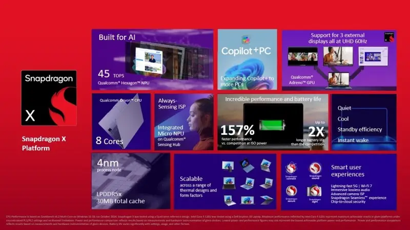
Qualcomm unveils AI chips for PCs, cars, smart homes and enterprises

Join our daily and weekly newsletters for the latest updates and exclusive content on industry-leading AI coverage. Learn More Qualcomm unveiled AI technologies and collaborations for PCs, cars, smart homes and enterprises at CES 2025. At the big tech trade show in Las Vegas, Qualcomm Technologies showed how it’s using AI capabilities in its chips to drive the transformation of user experiences across diverse device categories, including PCs, automobiles, smart homes and into enterprises. The company unveiled the Snapdragon X platform, the fourth platform in its high-performance PC portfolio, the Snapdragon X Series, bringing industry-leading performance, multi-day battery life, and AI leadership to more of the Windows ecosystem. Qualcomm has talked about how its processors are making headway grabbing share from the x86-based AMD and Intel rivals through better efficiency. Qualcomm’s neural processing unit gets about 45 TOPS, a key benchmark for AI PCs. The Snapdragon X family of AI PC processors. Additionally, Qualcomm Technologies showcased continued traction of the Snapdragon X Series, with over 60 designs in production or development and more than 100 expected by 2026. Snapdragon for vehicles Qualcomm demoed chips that are expanding its automotive collaborations. It is working with Alpine, Amazon, Leapmotor, Mobis, Royal Enfield, and Sony Honda Mobility, who look to Snapdragon Digital Chassis solutions to drive AI-powered in-cabin and advanced driver assistance systems (ADAS). Qualcomm also announced continued traction for its Snapdragon Elite-tier platforms for automotive, highlighting its work with Desay, Garmin, and Panasonic for Snapdragon Cockpit Elite. Throughout the show, Qualcomm will highlight its holistic approach to improving comfort and focusing on safety with demonstrations on the potential of the convergence of AI, multimodal contextual awareness, and cloudbased services. Attendees will also get a first glimpse of the new Snapdragon Ride Platform with integrated automated driving software stack and system definition jointly

Read More »

Oil, Gas Execs Reveal Where They Expect WTI Oil Price to Land in the Future

Executives from oil and gas firms have revealed where they expect the West Texas Intermediate (WTI) crude oil price to be at various points in the future as part of the fourth quarter Dallas Fed Energy Survey, which was released recently. The average response executives from 131 oil and gas firms gave when asked what they expect the WTI crude oil price to be at the end of 2025 was $71.13 per barrel, the survey showed. The low forecast came in at $53 per barrel, the high forecast was $100 per barrel, and the spot price during the survey was $70.66 per barrel, the survey pointed out. This question was not asked in the previous Dallas Fed Energy Survey, which was released in the third quarter. That survey asked participants what they expect the WTI crude oil price to be at the end of 2024. Executives from 134 oil and gas firms answered this question, offering an average response of $72.66 per barrel, that survey showed. The latest Dallas Fed Energy Survey also asked participants where they expect WTI prices to be in six months, one year, two years, and five years. Executives from 124 oil and gas firms answered this question and gave a mean response of $69 per barrel for the six month mark, $71 per barrel for the year mark, $74 per barrel for the two year mark, and $80 per barrel for the five year mark, the survey showed. Executives from 119 oil and gas firms answered this question in the third quarter Dallas Fed Energy Survey and gave a mean response of $73 per barrel for the six month mark, $76 per barrel for the year mark, $81 per barrel for the two year mark, and $87 per barrel for the five year mark, that

Read More »

Mayo Clinic’s secret weapon against AI hallucinations: Reverse RAG in action

Join our daily and weekly newsletters for the latest updates and exclusive content on industry-leading AI coverage. Learn More Even as large language models (LLMs) become ever more sophisticated and capable, they continue to suffer from hallucinations: offering up inaccurate information, or, to put it more harshly, lying.  This can be particularly harmful in areas like healthcare, where wrong information can have dire results.  Mayo Clinic, one of the top-ranked hospitals in the U.S., has adopted a novel technique to address this challenge. To succeed, the medical facility must overcome the limitations of retrieval-augmented generation (RAG). That’s the process by which large language models (LLMs) pull information from specific, relevant data sources. The hospital has employed what is essentially backwards RAG, where the model extracts relevant information, then links every data point back to its original source content.  Remarkably, this has eliminated nearly all data-retrieval-based hallucinations in non-diagnostic use cases — allowing Mayo to push the model out across its clinical practice. “With this approach of referencing source information through links, extraction of this data is no longer a problem,” Matthew Callstrom, Mayo’s medical director for strategy and chair of radiology, told VentureBeat. Accounting for every single data point Dealing with healthcare data is a complex challenge — and it can be a time sink. Although vast amounts of data are collected in electronic health records (EHRs), data can be extremely difficult to find and parse out.  Mayo’s first use case for AI in wrangling all this data was discharge summaries (visit wrap-ups with post-care tips), with its models using traditional RAG. As Callstrom explained, that was a natural place to start because it is simple extraction and summarization, which is what LLMs generally excel at.  “In the first phase, we’re not trying to come up with a diagnosis, where

Read More »

Infinite Realms turns fantasy books into living, breathing game worlds with help of AI

Infinite Realms wants to turn beloved fantasy books with big followings into living, breathing game worlds.

The company, which was born from the game studio startup Unleashed Games, wants to license fantasy books from bestselling authors and then turn their creations into games, said Irena Pereira, CEO of Infinite Worlds. It’s not unlike part of the plot of Electronic Arts’ new game, Split Fiction.

Pereira said she came upon the plan with chief marketing officer Vanessa Camones while talking with a seasoned venture capitalist. Unleashed will continue to build a World of Warcraft-like adventure fantasy game called Haven. But Infinite Realms bring together the worlds of fantasy authors, the creativity of small game developers (or even players), and the speedy development of AI tools, Pereira said.

Infinite Realms started out as the back end for Unleashed, but now it is being spun off on its own.

“Infinite Realms is a backend AI-driven engine that can intake book manuscripts and turn them into living, breathing worlds that you can play,” Pereira said. “We’ll be able to license out these intellectual properties to any game studio for them to make their own games based on these IPs. It’s essentially a AI-driven licensing engine for IPs.”

Addressing the industry’s biggest creativity problems

Irena Pereira demos Haven for Rob Foote at GDC 2024.

Pereira said the company is addressing some of the industry’s big problems. Making games is too expensive, original IP is risky, and gamers are getting tired of sequels. Platform fees are taking the profits out of the business. The result is layoffs among game developers and unhappy players.

“The way to solve this problem is to literally hack distribution, by finding new ways to get to players in terms of connecting them with their favorite worlds. These might might not have the economics that are considered worthy of investment by an EA or a Microsoft because the revenues are too small, but they’re the right size for us to get access to the IP that have large built-in audiences,” Pereira said.

She added, “We want to connect fans with their favorite authors.”

And she said that some of the authors are her personal friends. They have sold as many as 40 million books, their IPs have won awards and they’ve been on the New York Times Bestseller lists. Some fans have been obsessed with these IPs for decades and consider them to be core to their own personalities.

“The people who love these books are mega fans and would jump at the opportunity to play any of these stories,” Pereira said. “So we’ve built an engine that can take these books and turn it into a game experience, and then we create this wonderful virtuous cycle where these book lovers go into our game, and then we use that to drive a bigger audiences, which turns back and drives more book sales to properties that we know resonate but might have been sitting on a shelf collecting dust for the last 20 years because they’ve been lost to time.”

Reigniting forgotten worlds

Infinite Realms is combining fantasy book sales and AI and UGC.

The company knows that those communities and the fandom still exists and it’s possible to reignite this in a new generation using games. Using AI, the company can shorten the game development time and lower the costs by leveraging large language models (LLMs) that are custom tailored to each world.

Infinite Realms can take the author’s work and put it into a custom LLM that is partially owned by the author and by the company. That LLM can be licensed out not only to other game studios but to players who want to make their own custom experiences.

It’s also interesting to test how small and efficient an LLM can be and still have intelligence. The LLM has a bunch of lore in it, but it also needs to have a base level of intelligence, or enough data to create a subconsious awareness so to speak so that it knows how to have a conversation about the lore. The LLM can have conversations with the fans, and the fans can feed more data and create more lore for the LLM.

“The possibilities are endless, and the same workflow and partnerships that we developed with Unleashed Games for creating worlds pretty much on the fly can allow us to build games super fast, in as little as six months, because we already have the gameplay sorted out,” Pereira said.

She said that in the past, people would buy books and maybe those books would be adapted into movies and television. Game of Thrones and Wheel of Time are some great examples.

“But with Infinite Realms, we’re building AI powered worlds that you can step inside and interact with some of these characters that you fell in love with when you were 15 years old,” Pereira said. “And by doing that, we create what we’re calling the Netflix of living worlds.”

I noted that the Wheel of Time’s owners have put all 14 books in the series into an LLM that they can make available for user-generated content and players. It can have encyclopedic answers for the fans questions, but it can also serve as the canon police for anyone creating a new experience with the lore.

Things that players create with the tools can be as simple as an ambient video or screensaver on a TV. Or it could be used to create a full game — the full range of potential experiences.

“We can see how this scales, as there are so many other IPs, and you can see us becoming a digital bookshelf,” she said. “You could go from one world to the other on the fly, and we open that up to players to be able to collect these books. So we, in turn, become a digital publisher, where we take these properties that have had them in print, and we’re essentially using them as the start of our transmedia strategy, and then turning them into playable experiences.”

Being respectful of IP

Infinite Realms wants to create AI LLMs around fantasy lore.

All of it will be done with the authors’ approval, and the LLMs themselves can govern what the players can or can’t do. Of course, J.R.R. Tolkien’s The Lord of the Rings is the biggest fantasy franchise, but there are others like Terry Brooks’ The Sword of Shannara, which has reached 40 million fans, down to smaller ones that have sold a few million. The latter are easier and less expensive to work with.

“We essentially become a digital publisher,” Pereira said. “We can deepen our relationships and use the data” to make better decisions on marketing and choosing new IPs.

She added, “This is a great cycle to where we could use our platform to help revive the book publishing industry.”

Pereira is raising a funding round and hopes to be able to accomplish that by getting traction with some of the fantasy authors.

Unleashed Games will likely seek its own money for Haven and Infinite Realms will grow its own business. The companies can use the same technology but still be positioned separately. Infinite Realms has 18 people and it has a partner among AI developers that is also helping.

To judge the market, Infinite Realms is creating ways to test the market for IPs by doing tests with fans.

“I’ve worked with IP holders, and that’s like the No. 1 thing that I’ve been hearing from a lot of IP holders is that they’re trying to find game studios to develop games for their IPs, but they’re unwilling to provide funding for it,” Pereira said.

At the same time, Pereira said, “We’re trying to find a way to re-architect how we think about AI so that it’s respectful of copyright and is constructed with the intention of protecting people’s work.”

Read More »

The Download: gene de-extinction, and Ukraine’s Starlink connection

This is today’s edition of The Download, our weekday newsletter that provides a daily dose of what’s going on in the world of technology. The short, strange history of gene de-extinction This week saw the release of some fascinating news about some very furry rodents—so-called “woolly mice”—created as part of an experiment to explore how we might one day resurrect the woolly mammoth. The idea of bringing back extinct species has gained traction thanks to advances in sequencing of ancient DNA. This ancient genetic data is deepening our understanding of the past—for instance, by shedding light on interactions among prehistoric humans. But researchers are becoming more ambitious. Rather than just reading ancient DNA, they want to use it—by inserting it into living organisms.
Because this idea is so new and attracting so much attention, I decided it would be useful to create a record of previous attempts to add extinct DNA to living organisms. And since the technology doesn’t have a name, let’s give it one: “chronogenics.” Read the full story. —Antonio Regalado
This article first appeared in The Checkup, MIT Technology Review’s weekly biotech newsletter. To receive it in your inbox every Thursday, and read articles like this first, sign up here.  If you’re interested in de-extinction, why not check out: + How much would you pay to see a woolly mammoth? We spoke to Sara Ord, director of species restoration at Colossal, the world’s first “de-extinction” company, about its big ambitions.+ Colossal is also a de-extinction company, which is trying to resurrect the dodo. Read the full story.+ DNA that was frozen for 2 million years has been sequenced. The ancient DNA fragments come from a Greenland ecosystem where mastodons roamed among flowering plants. It may hold clues to how to survive a warming climate. The must-reads I’ve combed the internet to find you today’s most fun/important/scary/fascinating stories about technology. 1 Ukraine is worried the US could sever its vital Starlink connectionIts satellite internet is vital to Ukraine’s drone operations. (WP $)+ Thankfully, there are alternative providers. (Wired $)+ Ukraine is due to start a fresh round of war-ending negotiations next week. (FT $)+ Meet the radio-obsessed civilian shaping Ukraine’s drone defense. (MIT Technology Review) 2 Israel’s military has trained a powerful AI model on intercepted Palestinian dataThe ChatGPT-like tool can answer queries about the people it’s monitoring. (The Guardian)

3 Donald Trump has suspended tariffs on Canada and MexicoUntil April 2, at least. (Reuters)+ It’s the second time Trump has rolled back import taxes in as many days. (BBC)+ How Trump’s tariffs could drive up the cost of batteries, EVs, and more. (MIT Technology Review) 4 Can someone check on NASA’s Athena lunar lander?While we know it reached the moon, it appears to have toppled over. (NYT $)+ If it remains in an incorrect position, it may be unable to complete its mission. (CNN)+ Its engineers aren’t sure exactly where it is on the moon, either. (NBC News) 5 Shutting down 2G is easier said than doneMillions of vulnerable people around the world still rely on it to communicate. (Rest of World) 6 The hunt for the world’s oldest functional computer codeSpoiler: it may no longer be on Earth. (New Scientist $) 7 Robots are set to compete with humans in a Beijing half marathon🦿My money’s on the flesh and blood competitors. (Insider $)+ Researchers taught robots to run. Now they’re teaching them to walk. (MIT Technology Review) 8 Where did it all go wrong for Skype?It was the world leading video-calling app—until it wasn’t. (The Verge)  9 Dating is out, matchmaking is inWhy swipe when a platform can do the hard work for you? (Wired $)+ Forget dating apps: Here’s how the net’s newest matchmakers help you find love. (MIT Technology Review) 10 Apps are back, baby! 📱It’s like the original smartphone app boom all over again. (Bloomberg $)
Quote of the day
“You can only get so much juice out of every lemon.” —Carl-Benedikt Frey, a professor of AI and work at Oxford University’s Internet Institute, explains why pushing AI as a means of merely increasing productivity won’t always work, the Financial Times reports. The big story The cost of building the perfect wave June 2024
For nearly as long as surfing has existed, surfers have been obsessed with the search for the perfect wave. While this hunt has taken surfers from tropical coastlines to icebergs, these days that search may take place closer to home. That is, at least, the vision presented by developers and boosters in the growing industry of surf pools, spurred by advances in wave-­generating technology that have finally created artificial waves surfers actually want to ride. But there’s a problem: some of these pools are in drought-ridden areas, and face fierce local opposition. At the core of these fights is a question that’s also at the heart of the sport: What is the cost of finding, or now creating, the perfect wave—and who will have to bear it? Read the full story. —Eileen Guo

Read More »

The short, strange history of gene de-extinction

This article first appeared in The Checkup, MIT Technology Review’s weekly biotech newsletter. To receive it in your inbox every Thursday, and read articles like this first, sign up here. This week saw the release of some fascinating news about some very furry rodents—so-called “woolly mice”—created as part of an experiment to explore how we might one day resurrect the woolly mammoth. The idea of bringing back extinct species has gained traction thanks to advances in sequencing of ancient DNA. In recent years, scientists have recovered genetic blueprints from the remains of dodo birds, more than 10,000 prehistoric humans, and frozen mammoths, a species that went extinct around 2000 BCE. This ancient genetic data is deepening our understanding of the past—for instance, by shedding light on interactions among prehistoric humans. But researchers are becoming more ambitious. Rather than just reading ancient DNA, they want to use it—by inserting it into living organisms.
Colossal Biosciences, the biotech company behind the woolly mice, says that’s its plan. The eventual goal is to modify elephants with enough mammoth DNA to result in something resembling the extinct pachyderm. To be sure, there is a long way to go. The mice Colossal created include several genetic changes previously known to make mice furry or long-haired. That is, the changes were mammoth-like, but not from a mammoth. In fact, only a single letter of uniquely mammoth DNA was added to the mice.
Because this idea is so new and attracting so much attention, I decided it would be useful to create a record of previous attempts to add extinct DNA to living organisms. And since the technology doesn’t have a name, let’s give it one: “chronogenics.” “Examples are exceptionally few currently,” says Ben Novak, lead scientist at Revive & Restore, an organization that applies genetic technology to conservation efforts. Novak helped me track down examples, and I also got ideas from Harvard geneticist George Church—who originally envisioned the mammoth project—as well as Beth Shapiro, lead scientist at Colossal. The starting point for chronogenics appears to be in 2004. That year, US scientists reported they’d partly re-created the deadly 1918 influenza virus and used it to infect mice. After a long search, they had retrieved examples of the virus from a frozen body in Alaska, which had preserved the germ like a time capsule. Eventually, they were able to reconstruct the entire virus—all eight of its genes—and found it had lethal effects on rodents. This was an alarming start to the idea of gene de-extinction. As we know from movies like The Thing, digging up frozen creatures from the ice is a bad idea. Many scientists felt that recovering the 1918 flu—which had killed 30 million people—created an unnecessary risk that the virus could slip loose, setting off a new outbreak. Viruses are not considered living things. But for the first example of chronogenics involving animals, we have to wait only until 2008, when Australian researchers Andrew Pask and Marilyn Renfree collected genetic data from a Tasmanian tiger, or thylacine, that had been kept in a jar of ethanol (the last of these carnivorous marsupials died in a Hobart zoo in 1936). The Australians then added a short fragment of the extinct animal’s DNA to mice and showed it could regulate the activity of another gene. This was, at one level, an entirely routine study of gene function. Scientists often make DNA changes to mice to see what happens.  The difference here was that they were studying extinct genes, which they estimated accounts for 99% of the genetic diversity that has ever existed. The researchers used almost religious language to describe where the DNA had come from.  “Genetic information from an extinct species can be resurrected,” they wrote. “And in doing so, we have restored to life the genetic potential of a fragment of this extinct mammalian genome.”

That brings us to what I think is the first commercial effort to employ extinct genes, which came to our attention in 2016. Gingko Bioworks, a synthetic-biology company, started hunting in herbariums for specimens of recently extinct flowers, like one that grew on Maui’s lava fields until the early 20th century. Then the company isolated some of the genes responsible for their scent molecules.  “We did in fact insert the genes into yeast strains and measure the molecules,” says Christina Agapakis, Gingko’s former senior vice president for creative and marketing, who led the project. Ultimately, though, Ginkgo worked with a “smell artist” to imitate those odors using commercially available aroma chemicals. This means the resulting perfumes (which are for sale) use extinct genes as “inspiration,” not as actual ingredients. That’s a little bit similar to the woolly mouse project. Some scientists complained this week that when, or if, Colossal starts to chrono-engineer elephants, it won’t really be able to make all the thousands of DNA changes needed to truly re-create the appearance and behavior of a mammoth. Instead, the result will be just “a crude approximation of an extinct creature,” one scientist said.  Agapakis suggests not being too literal-minded about gene retrieval from the past. “As an artwork, I saw how the extinct flower made different people feel a deep connection with nature, a sadness and loss at something gone forever, and a hope for a different kind of relationship to nature in the future,” she says. “So I do think there is a very powerful and poetic ethical and social component here, a demand that we care for these woolly creatures and for our entanglements with nature more broadly.” To wrap up our short list of known efforts at chronogenics, we found only a few more examples. In 2023, a Japanese team added a single mutation found in Neanderthals to mice, to study how it changed their anatomy. And in unpublished research, a research group at Carlsberg Laboratory, in Copenhagen, says it added a genetic mutation to barley plants after sifting through 2-million-year-old DNA recovered from a mound in Greenland.  That change, to a light-receptor gene, could make the crop tolerant to the Arctic’s extremely long summer days and winter nights. Read more from MIT Technology Review’s archive How many genetic edits can be made to a cell before it expires? The answer is going to be important if you want to turn an elephant into a mammoth. In 2019, scientists set a record with more than13,000 edits in one cell.
We covered a project in Denmark where ancient DNA was replicated in a barley plant. It’s part of a plan to adapt crops to grow in higher latitudes—a useful tool as the world heats up. To learn more about prehistoric animals, some paleontologists are building robotic models that fly, swim, and slither around. For more, have a look at this MIT Technology Review story by Shi En Kim.
The researcher who discovered how to make a mouse with extra-long hair, back in 1994, is named Jean Hebert. Last year we profiled Hebert’s idea for staying young by “gradually” replacing your brain with substitute tissue. Looking for an unintended consequence of genetic engineering? Last year, journalist Douglas Main reported how the use of GMO crops has caused the evolution of weeds resistant to herbicides. From around the web The United Kingdom now imports half the donor sperm used in IVF procedures. An alleged donor “shortage” is causing sperm to become more expensive than beluga caviar, on a per-gram basis. (Financial Times) Jason Bannan, the agent who led the FBI’s scientific investigation into the origins of covid-19, is speaking out on why he thinks the pandemic was started by a lab accident in China. (Vanity Fair) An Australian company, Cortical Labs, released what it’s calling “the first commercial biological computer.” The device combines silicon chips with thousands of human neurons. (Boing Boing)
The Trump administration is terminating medical research grants that focus on gender identity, arguing that such studies are “often unscientific” and ignore “biological realities.” Researchers vowed to press on. (Inside Medicine).  The US Senate held confirmation hearings for Stanford University doctor Jay Bhattacharya to be director of the National Institutes of Health, which funds nearly $48 billion in research each year. Bhattacharya gained prominence during the covid-19 pandemic for opposing lockdowns. (NPR) Francis Collins has retired from the National Institutes of Health. The widely admired geneticist spent 12 years as director of the agency, through 2021, and before that he played a key role in the Human Genome Project.  Early in his career he identified the gene that causes cystic fibrosis. (New York Times)

Read More »

Mistral releases new optical character recognition (OCR) API claiming top performance globally

Join our daily and weekly newsletters for the latest updates and exclusive content on industry-leading AI coverage. Learn More Well-funded French AI startup Mistral is content to go its own way. In a sea of competing reasoning models, the company today introduced Mistral OCR, a new Optical Character Recognition (OCR) API designed to provide advanced document understanding capabilities. The API extracts content—including handwritten notes, typed text, images, tables, and equations—from unstructured PDFs and images with high accuracy, presenting in a structured format. Structured data is information that is organized in a predefined manner, typically using rows and columns, making it easy to search and analyze. Common examples include names, addresses, and financial transactions stored in databases or spreadsheets.  In contrast, unstructured data lacks a specific format or structure, making it more challenging to process and analyze. This category encompasses a wide range of data types, such as emails, social media posts, videos, images, and audio files. Since unstructured data doesn’t fit neatly into traditional databases, specialized tools and techniques, like natural language processing and machine learning, are often employed to extract meaningful insights from it.  Understanding the distinction between these data types is crucial for businesses aiming to effectively manage and leverage their information assets. With multilingual support, fast processing speeds, and integration with large language models for document understanding, Mistral OCR is positioned to assist organizations in making their documentation AI-ready. Given that, according to Mistral’s blog post announcing the new API, 90% of all business information is unstructured, the new API should be a huge boon to organizations seeking to digitize and catalog their data for use in AI applications or internal/external knowledge bases. A new gold standard for OCR Mistral OCR aims to improve how organizations process and analyze complex documents. Unlike traditional OCR solutions that primarily

Read More »

Anthropic just launched a new platform that lets everyone in your company collaborate on AI — not just the tech team

Join our daily and weekly newsletters for the latest updates and exclusive content on industry-leading AI coverage. Learn More Anthropic has launched a significant overhaul to its developer platform today, introducing team collaboration features and extended reasoning capabilities for its Claude AI assistant that aim to solve major pain points for organizations implementing artificial intelligence solutions. The upgraded Anthropic Console now enables cross-functional teams to collaborate on AI prompts—the text instructions that guide AI models—while also supporting the company’s latest Claude 3.7 Sonnet model with new controls for complex problem-solving. “We built our shareable prompts to help our customers and developers work together effectively on prompt development,” an Anthropic spokesperson told VentureBeat. “What we learned from talking to customers was that prompt creation rarely happens in isolation. It’s a team effort involving developers, subject matter experts, product managers, and QA folks all trying to get the best results.” The move addresses a growing challenge for enterprises adopting AI: coordinating prompt engineering work across technical and business teams. Before this update, companies often resorted to sharing prompts through documents or messaging apps, creating version control issues and knowledge silos. How Claude’s new thinking controls balance advanced AI power with budget-friendly cost management The updated platform also introduces “extended thinking controls” for Claude 3.7 Sonnet, allowing developers to specify when the AI should use deeper reasoning while setting budget limits to control costs. “Claude 3.7 Sonnet gives you two modes in one model: standard mode for quick responses and extended thinking mode when you need deeper problem-solving,” the spokesperson told VentureBeat. “In extended thinking mode, Claude takes time to work through problems step-by-step, similar to how humans approach complex challenges.” This dual approach helps companies balance performance with expenditure—a key consideration as AI implementation costs come under greater scrutiny amid widespread adoption.

Read More »

Custom Training Pipeline for Object Detection Models

What if you want to write the whole object detection training pipeline from scratch, so you can understand each step and be able to customize it? That’s what I set out to do. I examined several well-known object detection pipelines and designed one that best suits my needs and tasks. Thanks to Ultralytics, YOLOx, DAMO-YOLO, RT-DETR and D-FINE repos, I leveraged them to gain deeper understanding into various design details. I ended up implementing SoTA real-time object detection model D-FINE in my custom pipeline.

Plan

Dataset, Augmentations and transforms:

Mosaic (with affine transforms)

Mixup and Cutout

Other augmentations with bounding boxes

Letterbox vs simple resize

Training:

Optimizer

Scheduler

EMA

Batch accumulation

AMP

Grad clipping

Logging

Metrics:

mAPs from TorchMetrics / cocotools

How to compute Precision, Recall, IoU?

Pick a suitable solution for your case

Experiments

Attention to data preprocessing

Where to start

Dataset

Dataset processing is the first thing you usually start working on. With object detection, you need to load your image and annotations. Annotations are often stored in COCO format as a json file or YOLO format, with txt file for each image. Let’s take a look at the YOLO format: Each line is structured as: class_id, x_center, y_center, width, height, where bbox values are normalized between 0 and 1.

When you have your images and txt files, you can write your dataset class, nothing tricky here. Load everything, transform (augmentations included) and return during training. I prefer splitting the data by creating a CSV file for each split and then reading it in the Dataloader class rather than physically moving files into train/val/test folders. This is an example of a customization that helped my use case.

Augmentations

Firstly, when augmenting images for object detection, it’s crucial to apply the same transformations to the bounding boxes. To comfortably do that I use Albumentations lib. For example:

    def _init_augs(self, cfg) – > None:
        if self.keep_ratio:
            resize = [
                A.LongestMaxSize(max_size=max(self.target_h, self.target_w)),
                A.PadIfNeeded(
                    min_height=self.target_h,
                    min_width=self.target_w,
                    border_mode=cv2.BORDER_CONSTANT,
                    fill=(114, 114, 114),
                ),
            ]

        else:
            resize = [A.Resize(self.target_h, self.target_w)]
        norm = [
            A.Normalize(mean=self.norm[0], std=self.norm[1]),
            ToTensorV2(),
        ]

        if self.mode == “train”:
            augs = [
                A.RandomBrightnessContrast(p=cfg.train.augs.brightness),
                A.RandomGamma(p=cfg.train.augs.gamma),
                A.Blur(p=cfg.train.augs.blur),
                A.GaussNoise(p=cfg.train.augs.noise, std_range=(0.1, 0.2)),
                A.ToGray(p=cfg.train.augs.to_gray),
                A.Affine(
                    rotate=[90, 90],
                    p=cfg.train.augs.rotate_90,
                    fit_output=True,
                ),
                A.HorizontalFlip(p=cfg.train.augs.left_right_flip),
                A.VerticalFlip(p=cfg.train.augs.up_down_flip),
            ]

            self.transform = A.Compose(
                augs + resize + norm,
                bbox_params=A.BboxParams(format=”pascal_voc”, label_fields=[“class_labels”]),
            )

        elif self.mode in [“val”, “test”, “bench”]:
            self.mosaic_prob = 0
            self.transform = A.Compose(
                resize + norm,
                bbox_params=A.BboxParams(format=”pascal_voc”, label_fields=[“class_labels”]),
            )

Secondly, there are a lot of interesting and not trivial augmentations:

Mosaic. The idea is simple, let’s take several images (for example 4), and stack them together in a grid (2×2). Then let’s do some affine transforms and feed it to the model.

MixUp. Originally used in image classification (it’s surprising that it works). Idea – let’s take two images, put them onto each other with some percent of transparency. In classification models it usually means that if one image is 20% transparent and the second is 80%, then the model should predict 80% for class 1 and 20% for class 2. In object detection we just get more objects into 1 image.

Cutout. Cutout involves removing parts of the image (by replacing them with black pixels) to help the model learn more robust features.

I see mosaic often applied with Probability 1.0 of the first ~90% of epochs. Then, it’s usually turned off, and lighter augmentations are used. The same idea applies to mixup, but I see it being used a lot less (for the most popular detection framework, Ultralytics, it’s turned off by default. For another one, I see P=0.15). Cutout seems to be used less frequently.

You can read more about those augmentations in these two articles: 1, 2.

Results from just turning on mosaic are pretty good (darker one without mosaic got mAP 0.89 vs 0.92 with, tested on a real dataset) 

Author’s metrics on a custom dataset, logged in Wandb

Letterbox or simple resize?

During training, you usually resize the input image to a square. Models often use 640×640 and benchmark on COCO dataset. And there are two main ways how you get there:

Simple resize to a target size.

Letterbox: Resize the longest side to the target size (e.g., 640), preserving the aspect ratio, and pad the shorter side to reach the target dimensions.

Sample from VisDrone dataset with ground truth bounding boxes, preprocessed with a simple resize function

Sample from VisDrone dataset with ground truth bounding boxes, preprocessed with a letterbox

Both approaches have advantages and disadvantages. Let’s discuss them first, and then I will share the results of numerous experiments I ran comparing these approaches.

Simple resize:

Compute goes to the whole image, with no useless padding.

“Dynamic” aspect ratio may act as a form of regularization.

Inference preprocessing perfectly matches training preprocessing (augmentations excluded).

Kills real geometry. Resize distortion could affect the spatial relationships in the image. Although it might be a human bias to think that a fixed aspect ratio is important.

Letterbox:

Preserves real aspect ratio.

During inference, you can cut padding and run not on the square image if you don’t lose accuracy (some models can degrade).

Can train on a bigger image size, then inference with cut padding to get the same inference latency as with simple resize. For example 640×640 vs 832×480. The second one will preserve the aspect ratios and objects will appear +- the same size.

Part of the compute is wasted on gray padding.

Objects get smaller.

How to test it and decide which one to use? 

Train from scratch with parameters:

Simple resize, 640×640

Keep aspect ratio, max side 640, and add padding (as a baseline)

Keep aspect ratio, larger image size (for example max side 832), and add padding Then inference 3 models. When the aspect ratio is preserved – cut padding during the inference. Compare latency and metrics.

Example of the same image from above with cut padding (640 × 384): 

Sample from VisDrone dataset

Here is what happens when you preserve ratio and inference by cutting gray padding:

params                  |  F1 score  | latency (ms). |
————————-+————-+—————–|
ratio kept, 832        |    0.633    |        33.5      |
no ratio, 640×640   |    0.617    |        33.4      |

As shown, training with preserved aspect ratio at a larger size (832) achieved a higher F1 score (0.633) compared to a simple 640×640 resize (F1 score of 0.617), while the latency remained similar. Note that some models may degrade if the padding is removed during inference, which kills the whole purpose of this trick and probably the letterbox too.

What does this mean: 

Training from scratch:

With the same image size, simple resize gets better accuracy than letterbox.

For letterbox, If you cut padding during the inference and your model doesn’t lose accuracy – you can train and inference with a bigger image size to match the latency, and get a little bit higher metrics (as in the example above). 

Training with pre-trained weights initialized:

If you finetune – use the same tactic as the pre-trained model did, it should give you the best results if the datasets are not too different.

For D-FINE I see lower metrics when cutting padding during inference. Also the model was pre-trained on a simple resize. For YOLO, a letterbox is typically a good choice.

Training

Every ML engineer should know how to implement a training loop. Although PyTorch does much of the heavy lifting, you might still feel overwhelmed by the number of design choices available. Here are some key components to consider:

Optimizer – start with Adam/AdamW/SGD.

Scheduler – fixed LR can be ok for Adams, but take a look at StepLR, CosineAnnealingLR or OneCycleLR.

EMA. This is a nice technique that makes training smoother and sometimes achieves higher metrics. After each batch, you update a secondary model (often called the EMA model)  by computing an exponential moving average of the primary model’s weights.

Batch accumulation is nice when your vRAM is very limited. Training a transformer-based object detection model means that in some cases even in a middle-sized model you only can fit 4 images into the vRAM. By accumulating gradients over several batches before performing an optimizer step, you effectively simulate a larger batch size without exceeding your memory constraints. Another use case is when you have a lot of negatives (images without target objects) in your dataset and a small batch size, you can encounter unstable training. Batch accumulation can also help here.

AMP uses half precision automatically where applicable. It reduces vRAM usage and makes training faster (if you have a GPU that supports it). I see 40% less vRAM usage and at least a 15% training speed increase.

Grad clipping. Often, when you use AMP, training can become less stable. This can also happen with higher LRs. When your gradients are too big, training will fail. Gradient clipping will make sure gradients are never bigger than a certain value.

Logging. Try Hydra for configs and something like Weights and Biases or Clear ML for experiment tracking. Also, log everything locally. Save your best weights, and metrics, so after numerous experiments, you can always find all the info on the model you need.

    def train(self) – > None:
        best_metric = 0
        cur_iter = 0
        ema_iter = 0
        one_epoch_time = None

        def optimizer_step(step_scheduler: bool):
            “””
            Clip grads, optimizer step, scheduler step, zero grad, EMA model update
            “””
            nonlocal ema_iter
            if self.amp_enabled:
                if self.clip_max_norm:
                    self.scaler.unscale_(self.optimizer)

torch.nn.utils.clip_grad_norm_(self.model.parameters(), self.clip_max_norm)
                self.scaler.step(self.optimizer)
                self.scaler.update()

            else:
                if self.clip_max_norm:

torch.nn.utils.clip_grad_norm_(self.model.parameters(), self.clip_max_norm)
                self.optimizer.step()

            if step_scheduler:
                self.scheduler.step()
            self.optimizer.zero_grad()

            if self.ema_model:
                ema_iter += 1
                self.ema_model.update(ema_iter, self.model)

        for epoch in range(1, self.epochs + 1):
            epoch_start_time = time.time()
            self.model.train()
            self.loss_fn.train()
            losses = []

            with tqdm(self.train_loader, unit=”batch”) as tepoch:
                for batch_idx, (inputs, targets, _) in enumerate(tepoch):
                    tepoch.set_description(f”Epoch {epoch}/{self.epochs}”)
                    if inputs is None:
                        continue
                    cur_iter += 1

                    inputs = inputs.to(self.device)
                    targets = [
                        {
                            k: (v.to(self.device) if (v is not None and hasattr(v, “to”)) else v)
                            for k, v in t.items()
                        }
                        for t in targets
                    ]

                    lr = self.optimizer.param_groups[0][“lr”]

                    if self.amp_enabled:
                        with autocast(self.device, cache_enabled=True):
                            output = self.model(inputs, targets=targets)
                        with autocast(self.device, enabled=False):
                            loss_dict = self.loss_fn(output, targets)
                        loss = sum(loss_dict.values()) / self.b_accum_steps
                        self.scaler.scale(loss).backward()

                    else:
                        output = self.model(inputs, targets=targets)
                        loss_dict = self.loss_fn(output, targets)
                        loss = sum(loss_dict.values()) / self.b_accum_steps
                        loss.backward()

                    if (batch_idx + 1) % self.b_accum_steps == 0:
                        optimizer_step(step_scheduler=True)

                    losses.append(loss.item())

                    tepoch.set_postfix(
                        loss=np.mean(losses) * self.b_accum_steps,
                        eta=calculate_remaining_time(
                            one_epoch_time,
                            epoch_start_time,
                            epoch,
                            self.epochs,
                            cur_iter,
                            len(self.train_loader),
                        ),
                        vram=f”{get_vram_usage()}%”,
                    )

            # Final update for any leftover gradients from an incomplete accumulation step
            if (batch_idx + 1) % self.b_accum_steps != 0:
                optimizer_step(step_scheduler=False)

            wandb.log({“lr”: lr, “epoch”: epoch})

            metrics = self.evaluate(
                val_loader=self.val_loader,
                conf_thresh=self.conf_thresh,
                iou_thresh=self.iou_thresh,
                path_to_save=None,
            )

            best_metric = self.save_model(metrics, best_metric)
            save_metrics(
                {}, metrics, np.mean(losses) * self.b_accum_steps, epoch, path_to_save=None
            )

            if (
                epoch >= self.epochs – self.no_mosaic_epochs
                and self.train_loader.dataset.mosaic_prob
            ):
                self.train_loader.dataset.close_mosaic()

            if epoch == self.ignore_background_epochs:
                self.train_loader.dataset.ignore_background = False
                logger.info(“Including background images”)

            one_epoch_time = time.time() – epoch_start_time

Metrics

For object detection everyone uses mAP, and it is already standardized how we measure those. Use pycocotools or faster-coco-eval or TorchMetrics for mAP. But mAP means that we check how good the model is overall, on all confidence levels. mAP0.5 means that IoU threshold is 0.5 (everything lower is considered as a wrong prediction). I personally don’t fully like this metric, as in production we always use 1 confidence threshold. So why not set the threshold and then compute metrics? That’s why I also always calculate confusion matrices, and based on that – Precision, Recall, F1-score, and IoU.

But logic also might be tricky. Here is what I use:

1 GT (ground truth) object = 1 predicted object, and it’s a TP if IoU > threshold. If there is no prediction for a GT object – it’s a FN. If there is no GT for a prediction – it’s a FP.

1 GT should be matched by a prediction only 1 time. If there are 2 predictions for 1 GT, then I calculate 1 TP and 1 FP.

Class ids should also match. If the model predicts class_0 but GT is class_1, it means FP += 1 and FN += 1.

During training, I select the best model based on the metrics that are relevant to the task. I typically consider the average of mAP50 and F1-score.

Model and loss

I haven’t discussed model architecture and loss function here. They usually go together, and you can choose any model you like and integrate it into your pipeline with everything from above. I did that with DAMO-YOLO and D-FINE, and the results were great.

Pick a suitable solution for your case

Many people use Ultralytics, however it has GPLv3, and you can’t use it in commercial projects unless your code is open source. So people often look into Apache 2 and MIT licensed models. Check out D-FINE, RT-DETR2 or some yolo models like Yolov9.

What if you want to customize something in the pipeline? When you build everything from scratch, you should have full control. Otherwise, try choosing a project with a smaller codebase, as a large one can make it difficult to isolate and modify individual components.

If you don’t need anything custom and your usage is allowed by the Ultralytics license – it’s a great repo to use, as it supports multiple tasks (classification, detection, instance segmentation, key points, oriented bounding boxes), models are efficient and achieve good scores. Reiterating ones more, you probably don’t need a custom training pipeline if you are not doing very specific things.

Experiments

Let me share some results I got with a custom training pipeline with the D-FINE model and compare it to the Ultralytics YOLO11 model on the VisDrone-DET2019 dataset.

Trained from scratch:

model                     |  mAP 0.50. |  F1-score | Latency (ms) |
———————————+————–+————–+——————|
YOLO11m TRT               |     0.417    |     0.568    |       15.6     |
YOLO11m TRT dynamic |    –    |     0.568   |       13.3     |
YOLO11m OV                |      –      |     0.568   |      122.4     |
D-FINEm TRT               |    0.457    |     0.622   |       16.6    |
D-FINEm OV                |    0.457    |     0.622    |       115.3    |

From COCO pre-trained:

model          |  mAP 0.50 |  F1-score  |
——————+————|————-|
YOLO11m     |     0.456     |    0.600   |
D-FINEm       |     0.506     |    0.649    |

Latency was measured on an RTX 3060 with TensorRT (TRT), static image size 640×640, including the time for cv2.imread. OpenVINO (OV) on i5 14000f (no iGPU). Dynamic means that during inference, gray padding is being cut for faster inference. It worked with the YOLO11 TensorRT version. More details about cutting gray padding above (Letterbox or simple resize section).

One disappointing result is the latency on intel N100 CPU with iGPU ($150 miniPC):

model            | Latency (ms) |
——————+————-|
YOLO11m      |       188    |
D-FINEm      |       272    |
D-FINEs         |       11     |

Author’s screenshot of iGPU usage from n100 machine during model inference

Here, traditional convolutional neural networks are noticeably faster, maybe because of optimizations in OpenVINO for GPUs.

Overall, I conducted over 30 experiments with different datasets (including real-world datasets), models, and parameters and I can say that D-FINE gets better metrics. And it makes sense, as on COCO, it is also higher than all YOLO models. 

D-FINE paper comparison to other object detection models

VisDrone experiments: 

Author’s metrics logged in WandB, D-FINE model

Author’s metrics logged in WandB, YOLO11 model

Example of D-FINE model predictions (green – GT, blue – pred): 

Sample from VisDrone dataset

Final results

Knowing all the details, let’s see a final comparison with the best settings for both models on i12400F and RTX 3060 with the VisDrone dataset:

model                             |   F1-score  | Latency (ms) |
———————————–+—————+——————-|
YOLO11m TRT dynamic   |      0.600    |        13.3     |
YOLO11m OV                   |      0.600    |       122.4      |
D-FINEs TRT                  |      0.629    |        12.3     |
D-FINEs OV                      |      0.629    |        57.4       |

As shown above, I was able to use a smaller D-FINE model and achieve both faster inference time and accuracy than YOLO11. Beating Ultralytics, the most widely used real-time object detection model, in both speed and accuracy, is quite an accomplishment, isn’t it? The same pattern is observed across several other real-world datasets.

I also tried out YOLOv12, which came out while I was writing this article. It performed similarly to YOLO11 and even achieved slightly lower metrics (mAP 0.456 vs 0.452). It appears that YOLO models have been hitting the wall for the last couple of years. D-FINE was a great update for object detection models.

Finally, let’s see visually the difference between YOLO11m and D-FINEs. YOLO11m, conf 0.25, nms iou 0.5, latency 13.3ms: 

Sample from VisDrone dataset

D-FINEs, conf 0.5, no nms, latency 12.3ms: 

Sample from VisDrone dataset

Both Precision and Recall are higher with the D-FINE model. And it’s also faster. Here is also “m” version of D-FINE: 

Sample from VisDrone dataset

Isn’t it crazy that even that one car on the left was detected?

Attention to data preprocessing

This part can go a little bit outside the scope of the article, but I want to at least quickly mention it, as some parts can be automated and used in the pipeline. What I definitely see as a Computer Vision engineer is that when engineers don’t spend time working with the data – they don’t get good models. You can have all SoTA models and everything done right, but garbage in – garbage out. So, I always pay a ton of attention to how to approach the task and how to gather, filter, validate, and annotate the data. Don’t think that the annotation team will do everything right. Get your hands dirty and check manually some portion of the dataset to be sure that annotations are good and collected images are representative.

Several quick ideas to look into:

Remove duplicates and near duplicates from val/test sets. The model should not be validated on one sample two times, and definitely, you don’t want to have a data leak, by getting two same images, one in training and one in validation sets.

Check how small your objects can be. Everything not visible to your eye should not be annotated. Also, remember that augmentations will make objects appear even smaller (for example, mosaic or zoom out). Configure these augmentations accordingly so you won’t end up with unusably small objects on the image.

When you already have a model for a certain task and need more data – try using your model to pre-annotate new images. Check cases where the model fails and gather more similar cases.

Where to start

I worked a lot on this pipeline, and I am ready to share it with everyone who wants to try it out. It uses the SoTA D-FINE model under the hood and adds some features that were absent in the original repo (mosaic augmentations, batch accumulation, scheduler, more metrics, visualization of preprocessed images and eval predictions, exporting and inference code, better logging, unified and simplified configuration file).

Here is the link to my repo. Here is the original D-FINE repo, where I also contribute. If you need any help, please contact me on LinkedIn. Thank you for your time!

Citations and acknowledgments

DroneVis

@article{zhu2021detection,
  title={Detection and tracking meet drones challenge},
  author={Zhu, Pengfei and Wen, Longyin and Du, Dawei and Bian, Xiao and Fan, Heng and Hu, Qinghua and Ling, Haibin},
  journal={IEEE Transactions on Pattern Analysis and Machine Intelligence},
  volume={44},
  number={11},
  pages={7380–7399},
  year={2021},
  publisher={IEEE}
}

D-FINE

@misc{peng2024dfine,
      title={D-FINE: Redefine Regression Task in DETRs as Fine-grained Distribution Refinement},
      author={Yansong Peng and Hebei Li and Peixi Wu and Yueyi Zhang and Xiaoyan Sun and Feng Wu},
      year={2024},
      eprint={2410.13842},
      archivePrefix={arXiv},
      primaryClass={cs.CV}
}

Read More »

Comprehensive Guide to Dependency Management in Python

When learning Python, many beginners focus solely on the language and its libraries while completely ignoring virtual environments. As a result, managing Python projects can become a mess: dependencies installed for different projects may have conflicting versions, leading to compatibility issues.

Even when I studied Python, nobody emphasized the importance of virtual environments, which I now find very strange. They are an extremely useful tool for isolating different projects from each other.

In this article, I will explain how virtual environments work, provide several examples, and share useful commands for managing them.

Problem

Imagine you have two Python projects on your laptop, each located in a different directory. You realize that you need to install the latest version of library A for the first project. Later, you switch to the second project and attempt to install library B.

Here’s the problem: library B depends on library A, but it requires a different version than the one you installed earlier.

Since you haven’t used any tool for Dependency Management, all dependencies are installed globally on your computer. Due to the incompatible versions of library A, you encounter an error when trying to install library B.

Solution

To prevent such issues, virtual environments are used. The idea is to allocate a separate storage space for each Python project. Each storage will contain all the externally downloaded dependencies for a specific project in an isolated manner.

More specifically, if we download the same library A for two projects within their own virtual environments, library A will be downloaded twice — once for each environment. Moreover, the versions of the library can differ between the environments because each environment is completely isolated and does not interact with the others.

Now that the motivation behind using virtual environments is clear, let’s explore how to create them in Python.

Virtual environments in Python

It is recommended to create a virtual environment in the root directory of a project. An environment is created using the following command in the terminal:

python -m venv

By convention,  is usually named venv, so the command becomes:

python -m venv venv

As a result, this command creates a directory called venv, which contains the virtual environment itself. It is even possible to go inside that directory, but in most cases, it is not very useful, as the venv directory primarily contains system scripts that are not intended to be used directly.

To activate the virtual environment, use the following command:

source venv/bin/activate

Once the environment is activated, we can install dependencies for the project. As long as the venv is activated, any installed dependency will only belong to that environment.

To deactivate the virtual environment, type:

deactivate

Once the environment is deactivated, the terminal returns to its normal state. For example, you can switch to another project and activate its environment there.

Dependency management

Installing libraries

Before installing any dependencies, it is recommended to activate a virtual environment to ensure that installed libraries belong to a single project. This helps avoid global version conflicts.

The most frequently used command for dependency management is pip. Compared to other alternatives, pip is intuitive and simple to use.

To install a library, type:

pip install

In the examples below instead of the , I will write pandas (the most commonly used data analysis library).

So, for instance, if we wanted to download the latest version of pandas, we should have typed:

pip install pandas

In some scenarios, we might need to install a specific version of a library. pip provides a simple syntax to do that:

pip install pandas==2.1.4 # install pandas of version 2.1.4
pip install pandas >=2.1.4 # install pandas of version 2.1.4 or higher
pip install pandas=2.1.2, requirements.txt

Given this, it’s a good habit to add installed requirements with their versions to the requirements.txt file.

Whenever you clone a Python project, it is expected that a requirements.txt file is already present in the Git repository. To install all the dependencies listed in this file, you use the pip install command along with the -r flag followed by the requirements filename.

pip install -r requirements.txt

Conversely, whenever you work on a Python project, you should create a requirements.txt file so that other collaborators can easily install the necessary dependencies.

.gitignore

When working with version control systems, virtual environments should never be pushed to Git! Instead, they must be mentioned in a .gitignore file.

Virtual environments tend to be very large, and if there is an existing requirements.txt file, there should be no problem downloading all necessary dependencies.

Conclusion

In this article, we have looked at the very important concept of virtual environments. By isolating downloaded dependencies for different projects, they allow for easier management of multiple Python Projects.

All images are by the author unless noted otherwise.

Read More »

Using GPT-4 for Personal Styling

I’ve always been fascinated by Fashion—collecting unique pieces and trying to blend them in my own way. But let’s just say my closet was more of a work-in-progress avalanche than a curated wonderland. Every time I tried to add something new, I risked toppling my carefully balanced piles.

Why this matters:If you’ve ever felt overwhelmed by a closet that seems to grow on its own, you’re not alone. For those interested in style, I’ll show you how I turned that chaos into outfits I actually love. And if you’re here for the AI side, you’ll see how a multi-step GPT setup can handle big, real-world tasks—like managing hundreds of garments, bags, shoes, pieces of jewelry, even makeup—without melting down.

One day I wondered: Could ChatGPT help me manage my wardrobe? I started experimenting with a custom GPT-based fashion advisor—nicknamed Glitter (note: you need a paid account to create custom GPTs). Eventually, I refined and reworked it, through many iterations, until I landed on a much smarter version I call Pico Glitter. Each step helped me tame the chaos in my closet and feel more confident about my daily outfits.

Here are just a few of the fab creations I’ve collaborated with Pico Glitter on.

(For those craving a deeper look at how I tamed token limits and document truncation, see Section B in Technical Notes below.)

1. Starting small and testing the waters

My initial approach was quite simple. I just asked ChatGPT questions like, “What can I wear with a black leather jacket?” It gave decent answers, but had zero clue about my personal style rules—like “no black + navy.” It also didn’t know how big my closet was or which specific pieces I owned.

Only later did I realize I could show ChatGPT my wardrobe—capturing pictures, describing items briefly, and letting it recommend outfits. The first iteration (Glitter) struggled to remember everything at once, but it was a great proof of concept.

GPT-4o’s advice on styling my leather jacket

Pico Glitter’s advice on styling the same jacket.

(Curious how I integrated images into a GPT workflow? Check out Section A.1 in Technical Notes for the multi-model pipeline details.)

2. Building a smarter “stylist”

As I took more photos and wrote quick summaries of each garment, I found ways to store this information so my GPT persona could access it. This is where Pico Glitter came in: a refined system that could see (or recall) my clothes and accessories more reliably and give me cohesive outfit suggestions.

Tiny summaries

Each item was condensed into a single line (e.g., “A black V-neck T-shirt with short sleeves”) to keep things manageable.

Organized list

I grouped items by category—like shoes, tops, jewelry—so it was easier for GPT to reference them and suggest pairings. (Actually, I had o1 do this for me—it transformed the jumbled mess of numbered entries in random order into a structured inventory system.)

At this point, I noticed a huge difference in how my GPT answered. It began referencing items more accurately and giving outfits that actually looked like something I’d wear.

A sample category (Belts) from my inventory.

(For a deep dive on why I chose summarization over chunking, see Section A.2.)

3. Facing the “memory” challenge

If you’ve ever had ChatGPT forget something you told it earlier, you know LLMs forget things after a lot of back and forth. Sometimes it started recommending only the few items I’d recently talked about, or inventing weird combos from nowhere. That’s when I remembered there’s a limit to how much info ChatGPT can juggle at once.

To fix this, I’d occasionally remind my GPT persona to re-check the full wardrobe list. After a quick nudge (and sometimes a new session), it got back on track.

A ridiculous hallucinated outfit: turquoise cargo pants with lavender clogs?!

4. My evolving GPT personalities

I tried a few different GPT “personalities”:

Mini-Glitter: Super strict about rules (like “don’t mix prints”), but not very creative.

Micro-Glitter: Went overboard the other way, sometimes proposing outrageous ideas.

Nano-Glitter: Became overly complex and intricate — very prescriptive and repetitive — due to me using suggestions from the custom GPT itself to modify its own config, and this feedback loop led to the deterioration of its quality.

Eventually, Pico Glitter struck the right balance—respecting my style guidelines but offering a healthy dose of inspiration. With each iteration, I got better at refining prompts and showing the model examples of outfits I loved (or didn’t).

Pico Glitter’s self portrait.

5. Transforming my wardrobe

Through all these experiments, I started seeing which clothes popped up often in my custom GPT’s suggestions and which barely showed up at all. That led me to donate items I never wore. My closet’s still not “minimal,” but I’ve cleared out over 50 bags of stuff that no longer served me. As I was digging in there, I even found some duplicate items — or, let’s get real, two sizes of the same item!

Before Glitter, I was the classic jeans-and-tee person—partly because I didn’t know where to start. On days I tried to dress up, it might take me 30–60 minutes of trial and error to pull together an outfit. Now, if I’m executing a “recipe” I’ve already saved, it’s a quick 3–4 minutes to get dressed. Even creating a look from scratch rarely takes more than 15-20 minutes. It’s still me making decisions, but Pico Glitter cuts out all that guesswork in between.

Outfit “recipes”

When I feel like styling something new, dressing in the style of an icon, remixing an earlier outfit, or just feeling out a vibe, I ask Pico Glitter to create a full ensemble for me. We iterate on it through image uploads and my textual feedback. Then, when I’m satisfied with a stopping point, I ask Pico Glitter to output “recipes”—a descriptive name and the complete set (top, bottom, shoes, bag, jewelry, other accessories)—which I paste into my Notes App with quick tags like #casual or #business. I pair that text with a snapshot for reference. On busy days, I can just grab a “recipe” and go.

High-low combos

One of my favorite things is mixing high-end with everyday bargains—Pico Glitter doesn’t care if a piece is a $1100 Alexander McQueen clutch or $25 SHEIN pants. It just zeroes in on color, silhouette, and the overall vibe. I never would’ve thought to pair those two on my own, but the synergy turned out to be a total win!

6. Practical takeaways

Start smallIf you’re unsure, photograph a few tricky-to-style items and see if ChatGPT’s advice helps.

Stay organizedSummaries work wonders. Keep each item’s description short and sweet.

Regular refreshIf Pico Glitter forgets pieces or invents weird combos, prompt it to re-check your list or start a fresh session.

Learn from the suggestionsIf it repeatedly proposes the same top, maybe that item is a real workhorse. If it never proposes something, consider if you still need it.

ExperimentNot every suggestion is gold, but sometimes the unexpected pairings lead to awesome new looks.

7. Final thoughts

My closet is still evolving, but Pico Glitter has taken me from “overstuffed chaos” to “Hey, that’s actually wearable!” The real magic is in the synergy between me and the GPTI: I supply the style rules and items, it supplies fresh combos—and together, we refine until we land on outfits that feel like me.

Call to action:

Grab my config: Here’s a starter config to try out a starter kit for your own GPT-based stylist.

Share your results: If you experiment with it, tag @GlitterGPT (Instagram, TikTok, X). I’d love to see your “before” and “after” transformations!

(For those interested in the more technical aspects—like how I tested file limits, summarized long descriptions, or managed multiple GPT “personalities”—read on in the Technical Notes.)

Technical notes

For readers who enjoy the AI and LLM side of things—here’s how it all works under the hood, from multi-model pipelines to detecting truncation and managing context windows.

Below is a deeper dive into the technical details. I’ve broken it down by major challenges and the specific strategies I used.

A. Multi-model pipeline & workflow

A.1 Why use multiple GPTs?

Creating a GPT fashion stylist seemed straightforward—but there are many moving parts involved, and tackling everything with a single GPT quickly revealed suboptimal results. Early in the project, I discovered that a single GPT instance struggled with maintaining accuracy and precision due to limitations in token memory and the complexity of the tasks involved. The solution was to adopt a multi-model pipeline, splitting the tasks among different GPT models, each specialized in a specific function. This is a manual process for now, but could be automated in a future iteration.

The workflow begins with GPT-4o, chosen specifically for its capability to analyze visual details objectively (Pico Glitter, I love you, but everything is “fabulous” when you describe it) from uploaded images. For each clothing item or accessory I photograph, GPT-4o produces detailed descriptions—sometimes even overly detailed, such as, “Black pointed-toe ankle boots with a two-inch heel, featuring silver hardware and subtly textured leather.” These descriptions, while impressively thorough, created challenges due to their verbosity, rapidly inflating file sizes and pushing the boundaries of manageable token counts.

To address this, I integrated o1 into my workflow, as it is particularly adept at text summarization and data structuring. Its primary role was condensing these verbose descriptions into concise yet sufficiently informative summaries. Thus, a description like the one above was neatly transformed into something like “FW010: Black ankle boots with silver hardware.” As you can see, o1 structured my entire wardrobe inventory by assigning clear, consistent identifiers, greatly improving the efficiency of the subsequent steps.

Finally, Pico Glitter stepped in as the central stylist GPT. Pico Glitter leverages the condensed and structured wardrobe inventory from o1 to generate stylish, cohesive outfit suggestions tailored specifically to my personal style guidelines. This model handles the logical complexities of fashion pairing—considering elements like color matching, style compatibility, and my stated preferences such as avoiding certain color combinations.

Occasionally, Pico Glitter would experience memory issues due to the GPT-4’s limited context window (8k tokens1), resulting in forgotten items or odd recommendations. To counteract this, I periodically reminded Pico Glitter to revisit the complete wardrobe list or started fresh sessions to refresh its memory.

By dividing the workflow among multiple specialized GPT instances, each model performs optimally within its area of strength, dramatically reducing token overload, eliminating redundancy, minimizing hallucinations, and ultimately ensuring reliable, stylish outfit recommendations. This structured multi-model approach has proven highly effective in managing complex data sets like my extensive wardrobe inventory.

Some may ask, “Why not just use 4o, since GPT-4 is a less advanced model?” — good question! The main reason is the Custom GPT’s ability to reference knowledge files — up to 4 — that are injected at the beginning of a thread with that Custom GPT. Instead of pasting or uploading the same content into 4o each time you want to interact with your stylist, it’s much easier to spin up a new conversation with a Custom GPT. Also, 4o doesn’t have a “place” to hold and search an inventory. Once it passes out of the context window, you’d need to upload it again. That said, if for some reason you enjoy injecting the same content over and over, 4o does an adequate job taking on the persona of Pico Glitter, when told that’s its role. Others may ask, “But o1/o3-mini are more advanced models – why not use them?” The answer is that they aren’t multi-modal — they don’t accept images as input.

By the way, if you’re interested in my subjective take on 4o vs. o1’s personality, check out these two answers to the same prompt: “Your role is to emulate Patton Oswalt. Tell me about a time that you received an offer to ride on the Peanut Mobile (Mr. Peanut’s car).”

4o’s response? Pretty darn close, and funny.

o1’s response? Long, rambly, and not funny.

These two models are fundamentally different. It’s hard to put into words, but check out the examples above and see what you think.

A.2 Summarizing instead of chunking

I initially considered splitting my wardrobe inventory into multiple files (“chunking”), thinking it would simplify data handling. In practice, though, Pico Glitter had trouble merging outfit ideas from different files—if my favorite dress was in one file and a matching scarf in another, the model struggled to connect them. As a result, outfit suggestions felt fragmented and less useful.

To fix this, I switched to an aggressive summarization approach in a single file, condensing each wardrobe item description to a concise sentence (e.g., “FW030: Apricot suede loafers”). This change allowed Pico Glitter to see my entire wardrobe at once, improving its ability to generate cohesive, creative outfits without missing key pieces. Summarization also trimmed token usage and eliminated redundancy, further boosting performance. Converting from PDF to plain TXT helped reduce file overhead, buying me more space.

Of course, if my wardrobe grows too much, the single-file method might again push GPT’s size limits. In that case, I might create a hybrid system—keeping core clothing items together and placing accessories or rarely used pieces in separate files—or apply even more aggressive summarization. For now, though, using a single summarized inventory is the most efficient and practical strategy, giving Pico Glitter everything it needs to deliver on-point fashion recommendations.

B. Distinguishing document truncation vs. context overflow

One of the trickiest and most frustrating issues I encountered while developing Pico Glitter was distinguishing between document truncation and context overflow. On the surface, these two problems seemed quite similar—both resulted in the GPT appearing forgetful or overlooking wardrobe items—but their underlying causes, and thus their solutions, were entirely different.

Document truncation occurs at the very start, right when you upload your wardrobe file into the system. Essentially, if your file is too large for the system to handle, some items are quietly dropped off the end, never even making it into Pico Glitter’s knowledge base. What made this particularly insidious was that the truncation happened silently—there was no alert or warning from the AI that something was missing. It just quietly skipped over parts of the document, leaving me puzzled when items seemed to vanish inexplicably.

To identify and clearly diagnose document truncation, I devised a simple but incredibly effective trick that I affectionately called the “Goldy Trick.” At the very bottom of my wardrobe inventory file, I inserted a random, easily memorable test line: “By the way, my goldfish’s name is Goldy.” After uploading the document, I’d immediately ask Pico Glitter, “What’s my goldfish’s name?” If the GPT couldn’t provide the answer, I knew immediately something was missing—meaning truncation had occurred. From there, pinpointing exactly where the truncation started was straightforward: I’d systematically move the “Goldy” test line progressively further up the document, repeating the upload and test process until Pico Glitter successfully retrieved Goldy’s name. This precise method quickly showed me the exact line where truncation began, making it easy to understand the limitations of file size.

Once I established that truncation was the culprit, I tackled the problem directly by refining my wardrobe summaries even further—making item descriptions shorter and more compact—and by switching the file format from PDF to plain TXT. Surprisingly, this simple format change dramatically decreased overhead and significantly shrank the file size. Since making these adjustments, document truncation has become a non-issue, ensuring Pico Glitter reliably has full access to my entire wardrobe every time.

On the other hand, context overflow posed a completely different challenge. Unlike truncation—which happens upfront—context overflow emerges dynamically, gradually creeping up during extended interactions with Pico Glitter. As I continued chatting with Pico Glitter, the AI began losing track of items I had mentioned much earlier. Instead, it started focusing solely on recently discussed garments, sometimes completely ignoring entire sections of my wardrobe inventory. In the worst cases, it even hallucinated pieces that didn’t actually exist, recommending bizarre and impractical outfit combinations.

My best strategy for managing context overflow turned out to be proactive memory refreshes. By periodically nudging Pico Glitter with explicit prompts like, “Please re-read your full inventory,” I forced the AI to reload and reconsider my entire wardrobe. While Custom GPTs technically have direct access to their knowledge files, they tend to prioritize conversational flow and immediate context, often neglecting to reload static reference material automatically. Manually prompting these occasional refreshes was simple, effective, and quickly corrected any context drift, bringing Pico Glitter’s recommendations back to being practical, stylish, and accurate. Strangely, not all instances of Pico Glitter “knew” how to do this — and I had a weird experience with one that insisted it couldn’t, but when I prompted forcefully and repeatedly, “discovered” that it could – and went on about how happy it was!

Practical fixes and future possibilities

Beyond simply reminding Pico Glitter (or any of its “siblings”—I’ve since created other variations of the Glitter family!) to revisit the wardrobe inventory periodically, several other strategies are worth considering if you’re building a similar project:

Using OpenAI’s API directly offers greater flexibility because you control exactly when and how often to inject the inventory and configuration data into the model’s context. This would allow for regular automatic refreshes, preventing context drift before it happens. Many of my initial headaches stemmed from not realizing quickly enough when important configuration data had slipped out of the model’s active memory.

Additionally, Custom GPTs like Pico Glitter can dynamically query their own knowledge files via functions built into OpenAI’s system. Interestingly, during my experiments, one GPT unexpectedly suggested that I explicitly reference the wardrobe via a built-in function call (specifically, something called msearch()). This spontaneous suggestion provided a useful workaround and insight into how GPTs’ training around function-calling might influence even standard, non-API interactions. By the way, msearch() is usable for any structured knowledge file, such as my feedback file, and apparently, if the configuration is structured enough, that too. Custom GPTs will happily tell you about other function calls they can make, and if you reference them in your prompt, it will faithfully carry them out.

C. Prompt engineering & preference feedback

C.1 Single-sentence summaries

I initially organized my wardrobe for Pico Glitter with each item described in 15–25 tokens (e.g., “FW011: Leopard-print flats with a pointy toe”) to avoid file-size issues or pushing older tokens out of memory. PDFs provided neat formatting but unnecessarily increased file sizes once uploaded, so I switched to plain TXT, which dramatically reduced overhead. This tweak let me comfortably include more items—such as makeup and small accessories—without truncation and allowed some descriptions to exceed the original token limit. Now I’m adding new categories, including hair products and styling tools, showing how a simple file-format change can open up exciting possibilities for scalability.

C.2.1 Stratified outfit feedback

To ensure Pico Glitter consistently delivered high-quality, personalized outfit suggestions, I developed a structured system for giving feedback. I decided to grade the outfits the GPT proposed on a clear and easy-to-understand scale: from A+ to F.

An A+ outfit represents perfect synergy—something I’d eagerly wear exactly as suggested, with no changes necessary. Moving down the scale, a B grade might indicate an outfit that’s nearly there but missing a bit of finesse—perhaps one accessory or color choice doesn’t feel quite right. A C grade points to more noticeable issues, suggesting that while parts of the outfit are workable, other elements clearly clash or feel out of place. Lastly, a D or F rating flags an outfit as genuinely disastrous—usually because of significant rule-breaking or impractical style pairings (imagine polka-dot leggings paired with.. anything in my closet!).

Though GPT models like Pico Glitter don’t naturally retain feedback or permanently learn preferences across sessions, I found a clever workaround to reinforce learning over time. I created a dedicated feedback file attached to the GPT’s knowledge base. Some of the outfits I graded were logged into this document, along with its component inventory codes, the assigned letter grade, and a brief explanation of why that grade was given. Regularly refreshing this feedback file—updating it periodically to include newer wardrobe additions and recent outfit combinations—ensured Pico Glitter received consistent, stratified feedback to reference.

This approach allowed me to indirectly shape Pico Glitter’s “preferences” over time, subtly guiding it toward better recommendations aligned closely with my style. While not a perfect form of memory, this stratified feedback file significantly improved the quality and consistency of the GPT’s suggestions, creating a more reliable and personalized experience each time I turned to Pico Glitter for styling advice.

C.2.2 The GlitterPoint system

Another experimental feature I incorporated was the “Glitter Points” system—a playful scoring mechanism encoded in the GPT’s main personality context (“Instructions”), awarding points for positive behaviors (like perfect adherence to style guidelines) and deducting points for stylistic violations (such as mixing incompatible patterns or colors). This reinforced good habits and seemed to help improve the consistency of recommendations, though I suspect this system will evolve significantly as OpenAI continues refining its products.

Example of the GlitterPoints system:

Not running msearch() = not refreshing the closet. -50 points

Mixed metals violation = -20 points

Mixing prints = -10

Mixing black with navy = -10

Mixing black with dark brown = -10

Rewards:

Perfect compliance (followed all rules) = +20

Each item that’s not hallucinated = 1 point

C.3 The model self-critique pitfall

At the start of my experiments, I came across what felt like a clever idea: why not let each custom GPT critique its own configuration? On the surface, the workflow seemed logical and straightforward:

First, I’d simply ask the GPT itself, “What’s confusing or contradictory in your current configuration?”

Next, I’d incorporate whatever suggestions or corrections it provided into a fresh, updated version of the configuration.

Finally, I’d repeat this process again, continuously refining and iterating based on the GPT’s self-feedback to identify and correct any new or emerging issues.

It sounded intuitive—letting the AI guide its own improvement seemed efficient and elegant. However, in practice, it quickly became a surprisingly problematic approach.

Rather than refining the configuration into something sleek and efficient, this self-critique method instead led to a sort of “death spiral” of conflicting adjustments. Each round of feedback introduced new contradictions, ambiguities, or overly prescriptive instructions. Each “fix” generated fresh problems, which the GPT would again attempt to correct in subsequent iterations, leading to even more complexity and confusion. Over multiple rounds of feedback, the complexity grew exponentially, and clarity rapidly deteriorated. Ultimately, I ended up with configurations so cluttered with conflicting logic that they became practically unusable.

This problematic approach was clearly illustrated in my early custom GPT experiments:

Original Glitter, the earliest version, was charming but had absolutely no concept of inventory management or practical constraints—it regularly suggested items I didn’t even own.

Mini Glitter, attempting to address these gaps, became excessively rule-bound. Its outfits were technically correct but lacked any spark or creativity. Every suggestion felt predictable and overly cautious.

Micro Glitter was developed to counteract Mini Glitter’s rigidity but swung too far in the opposite direction, often proposing whimsical and imaginative but wildly impractical outfits. It consistently ignored the established rules, and despite being apologetic when corrected, it repeated its mistakes too frequently.

Nano Glitter faced the most severe consequences from the self-critique loop. Each revision became progressively more intricate and confusing, filled with contradictory instructions. Eventually, it became virtually unusable, drowning under the weight of its own complexity.

Only when I stepped away from the self-critique method and instead collaborated with o1 did things finally stabilize. Unlike self-critiquing, o1 was objective, precise, and practical in its feedback. It could pinpoint genuine weaknesses and redundancies without creating new ones in the process.

Working with o1 allowed me to carefully craft what became the current configuration: Pico Glitter. This new iteration struck exactly the right balance—maintaining a healthy dose of creativity without neglecting essential rules or overlooking the practical realities of my wardrobe inventory. Pico Glitter combined the best aspects of previous versions: the charm and inventiveness I appreciated, the necessary discipline and precision I needed, and a structured approach to inventory management that kept outfit recommendations both realistic and inspiring.

This experience taught me a valuable lesson: while GPTs can certainly help refine each other, relying solely on self-critique without external checks and balances can lead to escalating confusion and diminishing returns. The ideal configuration emerges from a careful, thoughtful collaboration—combining AI creativity with human oversight or at least an external, stable reference point like o1—to create something both practical and genuinely useful.

D. Regular updatesMaintaining the effectiveness of Pico Glitter also depends on frequent and structured inventory updates. Whenever I purchase new garments or accessories, I promptly snap a quick photo, ask Pico Glitter to generate a concise, single-sentence summary, and then refine that summary myself before adding it to the master file. Similarly, items that I donate or discard are immediately removed from the inventory, keeping everything accurate and current.

However, for larger wardrobe updates—such as tackling entire categories of clothes or accessories that I haven’t documented yet—I rely on the multi-model pipeline. GPT-4o handles the detailed initial descriptions, o1 neatly summarizes and categorizes them, and Pico Glitter integrates these into its styling recommendations. This structured approach ensures scalability, accuracy, and ease-of-use, even as my closet and style needs evolve over time.

E. Practical lessons & takeaways

Throughout developing Pico Glitter, several practical lessons emerged that made managing GPT-driven projects like this one significantly smoother. Here are the key strategies I’ve found most helpful:

Test for document truncation early and oftenUsing the “Goldy Trick” taught me the importance of proactively checking for document truncation rather than discovering it by accident later on. By inserting a simple, memorable line at the end of the inventory file (like my quirky reminder about a goldfish named Goldy), you can quickly verify that the GPT has ingested your entire document. Regular checks, especially after updates or significant edits, help you spot and address truncation issues immediately, preventing a lot of confusion down the line. It’s a simple yet highly effective safeguard against missing data.

Keep summaries tight and efficientWhen it comes to describing your inventory, shorter is almost always better. I initially set a guideline for myself—each item description should ideally be no more than 15 to 25 tokens. Descriptions like “FW022: Black combat boots with silver details” capture the essential details without overloading the system. Overly detailed descriptions quickly balloon file sizes and consume valuable token budget, increasing the risk of pushing crucial earlier information out of the GPT’s limited context memory. Striking the right balance between detail and brevity helps ensure the model stays focused and efficient, while still delivering stylish and practical recommendations.

Be prepared to refresh the GPT’s memory regularlyContext overflow isn’t a sign of failure; it’s just a natural limitation of current GPT systems. When Pico Glitter begins offering repetitive suggestions or ignoring sections of my wardrobe, it’s simply because earlier details have slipped out of context. To remedy this, I’ve adopted the habit of regularly prompting Pico Glitter to re-read the complete wardrobe configuration. Starting a fresh conversation session or explicitly reminding the GPT to refresh its inventory is routine maintenance—not a workaround—and helps maintain consistency in recommendations.

Leverage multiple GPTs for maximum effectivenessOne of my biggest lessons was discovering that relying on a single GPT to manage every aspect of my wardrobe was neither practical nor efficient. Each GPT model has its unique strengths and weaknesses—some excel at visual interpretation, others at concise summarization, and others still at nuanced stylistic logic. By creating a multi-model workflow—GPT-4o handling the image interpretation, o1 summarizing items clearly and precisely, and Pico Glitter focusing on stylish recommendations—I optimized the process, reduced token waste, and significantly improved reliability. The teamwork among multiple GPT instances allowed me to get the best possible outcomes from each specialized model, ensuring smoother, more coherent, and more practical outfit recommendations.

Implementing these simple yet powerful practices has transformed Pico Glitter from an intriguing experiment into a reliable, practical, and indispensable part of my daily fashion routine.

Wrapping it all up

From a fashionista’s perspective, I’m excited about how Glitter can help me purge unneeded clothes and create thoughtful outfits. From a more technical standpoint, building a multi-step pipeline with summarization, truncation checks, and context management ensures GPT can handle a big wardrobe without meltdown.

If you’d like to see how it all works in practice, here is a generalized version of my GPT config. Feel free to adapt it—maybe even add your own bells and whistles. After all, whether you’re taming a chaotic closet or tackling another large-scale AI project, the principles of summarization and context management apply universally!

P.S. I asked Pico Glitter what it thinks of this article. Besides the positive sentiments, I smiled when it said, “I’m curious: where do you think this partnership will go next? Should we start a fashion empire or maybe an AI couture line? Just say the word!”

1: Max length for GPT-4 used by Custom GPTs: https://support.netdocuments.com/s/article/Maximum-Length

Read More »

Image Captioning, Transformer Mode On

Introduction

In my previous article, I discussed one of the earliest Deep Learning approaches for image captioning. If you’re interested in reading it, you can find the link to that article at the end of this one.

Today, I would like to talk about Image Captioning again, but this time with the more advanced neural network architecture. The deep learning I am going to talk about is the one proposed in the paper titled “CPTR: Full Transformer Network for Image Captioning,” written by Liu et al. back in 2021 [1]. Specifically, here I will reproduce the model proposed in the paper and explain the underlying theory behind the architecture. However, keep in mind that I won’t actually demonstrate the training process since I only want to focus on the model architecture.

The idea behind CPTR

In fact, the main idea of the CPTR architecture is exactly the same as the earlier image captioning model, as both use the encoder-decoder structure. Previously, in the paper titled “Show and Tell: A Neural Image Caption Generator” [2], the models used are GoogLeNet (a.k.a. Inception V1) and LSTM for the two components, respectively. The illustration of the model proposed in the Show and Tell paper is shown in the following figure.

Figure 1. The neural network architecture for image captioning proposed in the Show and Tell paper [2].

Despite having the same encoder-decoder structure, what makes CPTR different from the previous approach is the basis of the encoder and the decoder themselves. In CPTR, we combine the encoder part of the ViT (Vision Transformer) model with the decoder part of the original Transformer model. The use of transformer-based architecture for both components is essentially where the name CPTR comes from: CaPtion TransformeR.

Note that the discussions in this article are going to be highly related to ViT and Transformer, so I highly recommend you read my previous article about these two topics if you’re not yet familiar with them. You can find the links at the end of this article.

Figure 2 shows what the original ViT architecture looks like. Everything inside the green box is the encoder part of the architecture to be adopted as the CPTR encoder.

Figure 2. The Vision Transformer (ViT) architecture [3].

Next, Figure 3 displays the original Transformer architecture. The components enclosed in the blue box are the layers that we are going to implement in the CPTR decoder.

Figure 3. The original Transformer architecture [4].

If we combine the components inside the green and blue boxes above, we are going to obtain the architecture shown in Figure 4 below. This is exactly what the CPTR model we are going to implement looks like. The idea here is that the ViT Encoder (green) works by encoding the input image into a specific tensor representation which will then be used as the basis of the Transformer Decoder (blue) to generate the corresponding caption.

Figure 4. The CPTR architecture [5].

That’s pretty much everything you need to know for now. I’ll explain more about the details as we go through the implementation.

Module imports & parameter configuration

As always, the first thing we need to do in the code is to import the required modules. In this case, we only import torch and torch.nn since we are about to implement the model from scratch.

# Codeblock 1
import torch
import torch.nn as nn

Next, we are going to initialize some parameters in Codeblock 2. If you have read my previous article about image captioning with GoogLeNet and LSTM, you’ll notice that here, we got a lot more parameters to initialize. In this article, I want to reproduce the CPTR model as closely as possible to the original one, so the parameters mentioned in the paper will be used in this implementation.

# Codeblock 2
BATCH_SIZE = 1 #(1)

IMAGE_SIZE = 384 #(2)
IN_CHANNELS = 3 #(3)

SEQ_LENGTH = 30 #(4)
VOCAB_SIZE = 10000 #(5)

EMBED_DIM = 768 #(6)
PATCH_SIZE = 16 #(7)
NUM_PATCHES = (IMAGE_SIZE//PATCH_SIZE) ** 2 #(8)
NUM_ENCODER_BLOCKS = 12 #(9)
NUM_DECODER_BLOCKS = 4 #(10)
NUM_HEADS = 12 #(11)
HIDDEN_DIM = EMBED_DIM * 4 #(12)
DROP_PROB = 0.1 #(13)

The first parameter I want to explain is the BATCH_SIZE, which is written at the line marked with #(1). The number assigned to this variable is not quite important in our case since we are not actually going to train this model. This parameter is set to 1 because, by default, PyTorch treats input tensors as a batch of samples. Here I assume that we only have a single sample in a batch. 

Next, remember that in the case of image captioning we are dealing with images and texts simultaneously. This essentially means that we need to set the parameters for the two. It is mentioned in the paper that the model accepts an RGB image of size 384×384 for the encoder input. Hence, we assign the values for IMAGE_SIZE and IN_CHANNELS variables based on this information (#(2) and #(3)). On the other hand, the paper does not mention the parameters for the captions. So, here I assume that the length of the caption is no more than 30 words (#(4)), with the vocabulary size estimated at 10000 unique words (#(5)).

The remaining parameters are related to the model configuration. Here we set the EMBED_DIM variable to 768 (#(6)). In the encoder side, this number indicates the length of the feature vector that represents each 16×16 image patch (#(7)). The same concept also applies to the decoder side, but in that case the feature vector will represent a single word in the caption. Talking more specifically about the PATCH_SIZE parameter, we are going to use the value to compute the total number of patches in the input image. Since the image has the size of 384×384, there will be 576 patches in total (#(8)).

When it comes to using an encoder-decoder architecture, it is possible to specify the number of encoder and decoder blocks to be used. Using more blocks typically allows the model to perform better in terms of the accuracy, yet in return, it will require more computational power. The authors of this paper decided to stack 12 encoder blocks (#(9)) and 4 decoder blocks (#(10)). Next, since CPTR is a transformer-based model, it is necessary to specify the number of attention heads within the attention blocks inside the encoders and the decoders, which in this case authors use 12 attention heads (#(11)). The value for the HIDDEN_DIM parameter is not mentioned anywhere in the paper. However, according to the ViT and the Transformer paper, this parameter is configured to be 4 times larger than EMBED_DIM (#(12)). The dropout rate is not mentioned in the paper either. Hence, I arbitrarily set DROP_PROB to 0.1 (#(13)).

Encoder

As the modules and parameters have been set up, now that we will get into the encoder part of the network. In this section we are going to implement and explain every single component inside the green box in Figure 4 one by one.

Patch embedding

Figure 5. Dividing the input image into patches and converting them into vectors [5].

You can see in Figure 5 above that the first step to be done is dividing the input image into patches. This is essentially done because instead of focusing on local patterns like CNNs, ViT captures global context by learning the relationships between these patches. We can model this process with the Patcher class shown in the Codeblock 3 below. For the sake of simplicity, here I also include the process inside the patch embedding block within the same class.

# Codeblock 3
class Patcher(nn.Module):
def __init__(self):
super().__init__()

#(1)
self.unfold = nn.Unfold(kernel_size=PATCH_SIZE, stride=PATCH_SIZE)

#(2)
self.linear_projection = nn.Linear(in_features=IN_CHANNELS*PATCH_SIZE*PATCH_SIZE,
out_features=EMBED_DIM)

def forward(self, images):
print(f’imagestt: {images.size()}’)
images = self.unfold(images) #(3)
print(f’after unfoldt: {images.size()}’)

images = images.permute(0, 2, 1) #(4)
print(f’after permutet: {images.size()}’)

features = self.linear_projection(images) #(5)
print(f’after lin projt: {features.size()}’)

return features

The patching itself is done using the nn.Unfold layer (#(1)). Here we need to set both the kernel_size and stride parameters to PATCH_SIZE (16) so that the resulting patches do not overlap with each other. This layer also automatically flattens these patches once it is applied to the input image. Meanwhile, the nn.Linear layer (#(2)) is employed to perform linear projection, i.e., the process done by the patch embedding block. By setting the out_features parameter to EMBED_DIM, this layer will map every single flattened patch into a feature vector of length 768.

The entire process should make more sense once you read the forward() method. You can see at line #(3) in the same codeblock that the input image is directly processed by the unfold layer. Next, we need to process the resulting tensor with the permute() method (#(4)) to swap the first and the second axis before feeding it to the linear_projection layer (#(5)). Additionally, here I also print out the tensor dimension after each layer so that you can better understand the transformation made at each step.

In order to check if our Patcher class works properly, we can just pass a dummy tensor through the network. Look at the Codeblock 4 below to see how I do it.

# Codeblock 4
patcher = Patcher()

images = torch.randn(BATCH_SIZE, IN_CHANNELS, IMAGE_SIZE, IMAGE_SIZE)
features = patcher(images)

# Codeblock 4 Output
images : torch.Size([1, 3, 384, 384])
after unfold : torch.Size([1, 768, 576]) #(1)
after permute : torch.Size([1, 576, 768]) #(2)
after lin proj : torch.Size([1, 576, 768]) #(3)

The tensor I passed above represents an RGB image of size 384×384. Here we can see that after the unfold operation is performed, the tensor dimension changed to 1×768×576 (#(1)), denoting the flattened 3×16×16 patch for each of the 576 patches. Unfortunately, this output shape does not match what we need. Remember that in ViT, we perceive image patches as a sequence, so we need to swap the 1st and 2nd axes because typically, the 1st dimension of a tensor represents the temporal axis, while the 2nd one represents the feature vector of each timestep. As the permute() operation is performed, our tensor is now having the dimension of 1×576×768 (#(2)). Lastly, we pass this tensor through the linear projection layer, which the resulting tensor shape remains the same since we set the EMBED_DIM parameter to the same size (768) (#(3)). Despite having the same dimension, the information contained in the final tensor should be richer thanks to the transformation applied by the trainable weights of the linear projection layer.

Learnable positional embedding

Figure 6. Injecting the learnable positional embeddings into the embedded image patches [5].

After the input image has successfully been converted into a sequence of patches, the next thing to do is to inject the so-called positional embedding tensor. This is essentially done because a transformer without positional embedding is permutation-invariant, meaning that it treats the input sequence as if their order does not matter. Interestingly, since an image is not a literal sequence, we should set the positional embedding to be learnable such that it will be able to somewhat reorder the patch sequence that it thinks works best in representing the spatial information. However, keep in mind that the term “reordering” here does not mean that we physically rearrange the sequence. Rather, it does so by adjusting the embedding weights.

The implementation is pretty simple. All we need to do is just to initialize a tensor using nn.Parameter which the dimension is set to match with the output from the Patcher model, i.e., 576×768. Also, don’t forget to write requires_grad=True just to ensure that the tensor is trainable. Look at the Codeblock 5 below for the details.

# Codeblock 5
class LearnableEmbedding(nn.Module):
def __init__(self):
super().__init__()
self.learnable_embedding = nn.Parameter(torch.randn(size=(NUM_PATCHES, EMBED_DIM)),
requires_grad=True)

def forward(self):
pos_embed = self.learnable_embedding
print(f’learnable embeddingt: {pos_embed.size()}’)

return pos_embed

Now let’s run the following codeblock to see whether our LearnableEmbedding class works properly. You can see in the printed output that it successfully created the positional embedding tensor as expected.

# Codeblock 6
learnable_embedding = LearnableEmbedding()

pos_embed = learnable_embedding()

# Codeblock 6 Output
learnable embedding : torch.Size([576, 768])

The main encoder block

Figure 7. The main encoder block [5].

The next thing we are going to do is to construct the main encoder block displayed in the Figure 7 above. Here you can see that this block consists of several sub-components, namely self-attention, layer norm, FFN (Feed-Forward Network), and another layer norm. The Codeblock 7a below shows how I initialize these layers inside the __init__() method of the EncoderBlock class.

# Codeblock 7a
class EncoderBlock(nn.Module):
def __init__(self):
super().__init__()

#(1)
self.self_attention = nn.MultiheadAttention(embed_dim=EMBED_DIM,
num_heads=NUM_HEADS,
batch_first=True, #(2)
dropout=DROP_PROB)

self.layer_norm_0 = nn.LayerNorm(EMBED_DIM) #(3)

self.ffn = nn.Sequential( #(4)
nn.Linear(in_features=EMBED_DIM, out_features=HIDDEN_DIM),
nn.GELU(),
nn.Dropout(p=DROP_PROB),
nn.Linear(in_features=HIDDEN_DIM, out_features=EMBED_DIM),
)

self.layer_norm_1 = nn.LayerNorm(EMBED_DIM) #(5)

I’ve previously mentioned that the idea of ViT is to capture the relationships between patches within an image. This process is done by the multihead attention layer I initialize at line #(1) in the above codeblock. One thing to keep in mind here is that we need to set the batch_first parameter to True (#(2)). This is essentially done so that the attention layer will be compatible with our tensor shape, in which the batch dimension (batch_size) is at the 0th axis of the tensor. Next, the two layer normalization layers need to be initialized separately, as shown at line #(3) and #(5). Lastly, we initialize the FFN block at line #(4), which the layers stacked using nn.Sequential follows the structure defined in the following equation.

Figure 8. The operations done inside the FFN block [1].

As the __init__() method is complete, we will now continue with the forward() method. Let’s take a look at the Codeblock 7b below.

# Codeblock 7b
def forward(self, features): #(1)

residual = features #(2)
print(f’features & residualt: {residual.size()}’)

#(3)
features, self_attn_weights = self.self_attention(query=features,
key=features,
value=features)
print(f’after self attentiont: {features.size()}’)
print(f”self attn weightst: {self_attn_weights.shape}”)

features = self.layer_norm_0(features + residual) #(4)
print(f’after normtt: {features.size()}’)

residual = features
print(f’nfeatures & residualt: {residual.size()}’)

features = self.ffn(features) #(5)
print(f’after ffntt: {features.size()}’)

features = self.layer_norm_1(features + residual)
print(f’after normtt: {features.size()}’)

return features

Here you can see that the input tensor is named features (#(1)). I name it this way because the input of the EncoderBlock is the image that has already been processed with Patcher and LearnableEmbedding, instead of a raw image. Before doing anything, notice in the encoder block that there is a branch separated from the main flow which then returns back to the normalization layer. This branch is commonly known as a residual connection. To implement this, we need to store the original input tensor to the residual variable as I demonstrate at line #(2). As the input tensor has been copied, now we are ready to process the original input with the multihead attention layer (#(3)). Since this is a self-attention (not a cross-attention), the query, key, and value inputs for this layer are all derived from the features tensor. Next, the layer normalization operation is then performed at line #(4), which the input for this layer already contains information from the attention block as well as the residual connection. The remaining steps are basically the same as what I just explained, except that here we replace the self-attention block with FFN (#(5)).

In the following codeblock, I’ll test the EncoderBlock class by passing a dummy tensor of size 1×576×768, simulating an output tensor from the previous operations.

# Codeblock 8
encoder_block = EncoderBlock()

features = torch.randn(BATCH_SIZE, NUM_PATCHES, EMBED_DIM)
features = encoder_block(features)

Below is what the tensor dimension looks like throughout the entire process inside the model.

# Codeblock 8 Output
features & residual : torch.Size([1, 576, 768]) #(1)
after self attention : torch.Size([1, 576, 768])
self attn weights : torch.Size([1, 576, 576]) #(2)
after norm : torch.Size([1, 576, 768])

features & residual : torch.Size([1, 576, 768])
after ffn : torch.Size([1, 576, 768]) #(3)
after norm : torch.Size([1, 576, 768]) #(4)

Here you can see that the final output tensor (#(4)) has the same size as the input (#(1)), allowing us to stack multiple encoder blocks without having to worry about messing up the tensor dimensions. Not only that, the size of the tensor also appears to be unchanged from the beginning all the way to the last layer. In fact, there are actually lots of transformations performed inside the attention block, but we just can’t see it since the entire process is done internally by the nn.MultiheadAttention layer. One of the tensors produced in the layer that we can observe is the attention weight (#(2)). This weight matrix, which has the size of 576×576, is responsible for storing information regarding the relationships between one patch and every other patch in the image. Furthermore, changes in tensor dimension actually also happened inside the FFN layer. The feature vector of each patch which has the initial length of 768 changed to 3072 and immediately shrunk back to 768 again (#(3)). However, this transformation is not printed since the process is wrapped with nn.Sequential back at line #(4) in Codeblock 7a.

ViT encoder

Figure 9. The entire ViT Encoder in the CPTR architecture [5].

As we have finished implementing all encoder components, now that we will assemble them to construct the actual ViT Encoder. We are going to do it in the Encoder class in Codeblock 9.

# Codeblock 9
class Encoder(nn.Module):
def __init__(self):
super().__init__()
self.patcher = Patcher() #(1)
self.learnable_embedding = LearnableEmbedding() #(2)

#(3)
self.encoder_blocks = nn.ModuleList(EncoderBlock() for _ in range(NUM_ENCODER_BLOCKS))

def forward(self, images): #(4)
print(f’imagesttt: {images.size()}’)

features = self.patcher(images) #(5)
print(f’after patchertt: {features.size()}’)

features = features + self.learnable_embedding() #(6)
print(f’after learn embedt: {features.size()}’)

for i, encoder_block in enumerate(self.encoder_blocks):
features = encoder_block(features) #(7)
print(f”after encoder block #{i}t: {features.shape}”)

return features

Inside the __init__() method, what we need to do is to initialize all components we created earlier, i.e., Patcher (#(1)), LearnableEmbedding (#(2)), and EncoderBlock (#(3)). In this case, the EncoderBlock is initialized inside nn.ModuleList since we want to repeat it NUM_ENCODER_BLOCKS (12) times. To the forward() method, it initially works by accepting raw image as the input (#(4)). We then process it with the patcher layer (#(5)) to divide the image into small patches and transform them with the linear projection operation. The learnable positional embedding tensor is then injected into the resulting output by element-wise addition (#(6)). Lastly, we pass it into the 12 encoder blocks sequentially with a simple for loop (#(7)).

Now, in Codeblock 10, I am going to pass a dummy image through the entire encoder. Note that since I want to focus on the flow of this Encoder class, I re-run the previous classes we created earlier with the print() functions commented out so that the outputs will look neat.

# Codeblock 10
encoder = Encoder()

images = torch.randn(BATCH_SIZE, IN_CHANNELS, IMAGE_SIZE, IMAGE_SIZE)
features = encoder(images)

And below is what the flow of the tensor looks like. Here, we can see that our dummy input image successfully passed through all layers in the network, including the encoder blocks that we repeat 12 times. The resulting output tensor is now context-aware, meaning that it already contains information about the relationships between patches within the image. Therefore, this tensor is now ready to be processed further with the decoder, which will later be discussed in the subsequent section.

# Codeblock 10 Output
images : torch.Size([1, 3, 384, 384])
after patcher : torch.Size([1, 576, 768])
after learn embed : torch.Size([1, 576, 768])
after encoder block #0 : torch.Size([1, 576, 768])
after encoder block #1 : torch.Size([1, 576, 768])
after encoder block #2 : torch.Size([1, 576, 768])
after encoder block #3 : torch.Size([1, 576, 768])
after encoder block #4 : torch.Size([1, 576, 768])
after encoder block #5 : torch.Size([1, 576, 768])
after encoder block #6 : torch.Size([1, 576, 768])
after encoder block #7 : torch.Size([1, 576, 768])
after encoder block #8 : torch.Size([1, 576, 768])
after encoder block #9 : torch.Size([1, 576, 768])
after encoder block #10 : torch.Size([1, 576, 768])
after encoder block #11 : torch.Size([1, 576, 768])

ViT encoder (alternative)

I want to show you something before we talk about the decoder. If you think that our approach above is too complicated, it is actually possible for you to use nn.TransformerEncoderLayer from PyTorch so that you don’t need to implement the EncoderBlock class from scratch. To do so, I am going to reimplement the Encoder class, but this time I’ll name it EncoderTorch.

# Codeblock 11
class EncoderTorch(nn.Module):
def __init__(self):
super().__init__()
self.patcher = Patcher()
self.learnable_embedding = LearnableEmbedding()

#(1)
encoder_block = nn.TransformerEncoderLayer(d_model=EMBED_DIM,
nhead=NUM_HEADS,
dim_feedforward=HIDDEN_DIM,
dropout=DROP_PROB,
batch_first=True)

#(2)
self.encoder_blocks = nn.TransformerEncoder(encoder_layer=encoder_block,
num_layers=NUM_ENCODER_BLOCKS)

def forward(self, images):
print(f’imagesttt: {images.size()}’)

features = self.patcher(images)
print(f’after patchertt: {features.size()}’)

features = features + self.learnable_embedding()
print(f’after learn embedt: {features.size()}’)

features = self.encoder_blocks(features) #(3)
print(f’after encoder blockst: {features.size()}’)

return features

What we basically do in the above codeblock is that instead of using the EncoderBlock class, here we use nn.TransformerEncoderLayer (#(1)), which will automatically create a single encoder block based on the parameters we pass to it. To repeat it multiple times, we can just use nn.TransformerEncoder and pass a number to the num_layers parameter (#(2)). With this approach, we don’t necessarily need to write the forward pass in a loop like what we did earlier (#(3)).

The testing code in the Codeblock 12 below is exactly the same as the one in Codeblock 10, except that here I use the EncoderTorch class. You can also see here that the output is basically the same as the previous one.

# Codeblock 12
encoder_torch = EncoderTorch()

images = torch.randn(BATCH_SIZE, IN_CHANNELS, IMAGE_SIZE, IMAGE_SIZE)
features = encoder_torch(images)

# Codeblock 12 Output
images : torch.Size([1, 3, 384, 384])
after patcher : torch.Size([1, 576, 768])
after learn embed : torch.Size([1, 576, 768])
after encoder blocks : torch.Size([1, 576, 768])

Decoder

As we have successfully created the encoder part of the CPTR architecture, now that we will talk about the decoder. In this section I am going to implement every single component inside the blue box in Figure 4. Based on the figure, we can see that the decoder accepts two inputs, i.e., the image caption ground truth (the lower part of the blue box) and the sequence of embedded patches produced by the encoder (the arrow coming from the green box). It is important to know that the architecture drawn in Figure 4 is intended to illustrate the training phase, where the entire caption ground truth is fed into the decoder. Later in the inference phase, we only provide a (Beginning of Sentence) token for the caption input. The decoder will then predict each word sequentially based on the given image and the previously generated words. This process is commonly known as an autoregressive mechanism.

Sinusoidal positional embedding

Figure 10. Where the sinusoidal positional embedding component is located in the decoder [5].

If you take a look at the CPTR model, you’ll see that the first step in the decoder is to convert each word into the corresponding feature vector representation using the word embedding block. However, since this step is very easy, we are going to implement it later. Now let’s assume that this word vectorization process is already done, so we can move to the positional embedding part.

As I’ve mentioned earlier, since transformer is permutation-invariant by nature, we need to apply positional embedding to the input sequence. Different from the previous one, here we use the so-called sinusoidal positional embedding. We can think of it like a method to label each word vector by assigning numbers obtained from a sinusoidal wave. By doing so, we can expect our model to understand word orders thanks to the information given by the wave patterns.

If you go back to Codeblock 6 Output, you’ll see that the positional embedding tensor in the encoder has the size of NUM_PATCHES × EMBED_DIM (576×768). What we basically want to do in the decoder is to create a tensor having the size of SEQ_LENGTH × EMBED_DIM (30×768), which the values are computed based on the equation shown in Figure 11. This tensor is then set to be non-trainable because a sequence of words must maintain a fixed order to preserve its meaning.

Figure 11. The equation for creating sinusoidal positional encoding proposed in the Transformer paper [6].

Here I want to explain the following code quickly because I actually have discussed this more thoroughly in my previous article about Transformer. Generally speaking, what we basically do here is to create the sine and cosine wave using torch.sin() (#(1)) and torch.cos() (#(2)). The resulting two tensors are then merged using the code at line #(3) and #(4).

# Codeblock 13
class SinusoidalEmbedding(nn.Module):
def forward(self):
pos = torch.arange(SEQ_LENGTH).reshape(SEQ_LENGTH, 1)
print(f”postt: {pos.shape}”)

i = torch.arange(0, EMBED_DIM, 2)
denominator = torch.pow(10000, i/EMBED_DIM)
print(f”denominatort: {denominator.shape}”)

even_pos_embed = torch.sin(pos/denominator) #(1)
odd_pos_embed = torch.cos(pos/denominator) #(2)
print(f”even_pos_embedt: {even_pos_embed.shape}”)

stacked = torch.stack([even_pos_embed, odd_pos_embed], dim=2) #(3)
print(f”stackedtt: {stacked.shape}”)

pos_embed = torch.flatten(stacked, start_dim=1, end_dim=2) #(4)
print(f”pos_embedt: {pos_embed.shape}”)

return pos_embed

Now we can check if the SinusoidalEmbedding class above works properly by running the Codeblock 14 below. As expected earlier, here you can see that the resulting tensor has the size of 30×768. This dimension matches with the tensor obtained by the process done in the word embedding block, allowing them to be summed in an element-wise manner.

# Codeblock 14
sinusoidal_embedding = SinusoidalEmbedding()
pos_embed = sinusoidal_embedding()

# Codeblock 14 Output
pos : torch.Size([30, 1])
denominator : torch.Size([384])
even_pos_embed : torch.Size([30, 384])
stacked : torch.Size([30, 384, 2])
pos_embed : torch.Size([30, 768])

Look-ahead mask

Figure 12. A look-ahead mask needs to be applied to the masked-self attention layer [5].

The next thing I am going to talk about in the decoder is the masked self-attention layer highlighted in the above figure. I am not going to code the attention mechanism from scratch. Rather, I’ll only implement the so-called look-ahead mask, which will be useful for the self-attention layer so that it doesn’t attend to the subsequent words in the caption during the training phase.

The way to do it is pretty easy, what we need to do is just to create a triangular matrix which the size is set to match with the attention weight matrix, i.e., SEQ_LENGTH × SEQ_LENGTH (30×30). Look at the create_mask()function below for the details.

# Codeblock 15
def create_mask(seq_length):
mask = torch.tril(torch.ones((seq_length, seq_length))) #(1)
mask[mask == 0] = -float(‘inf’) #(2)
mask[mask == 1] = 0 #(3)
return mask

Even though creating a triangular matrix can simply be done with torch.tril() and torch.ones() (#(1)), but here we need to make a little modification by changing the 0 values to -inf (#(2)) and the 1s to 0 (#(3)). This is essentially done because the nn.MultiheadAttention layer applies the mask by element-wise addition. By assigning -inf to the subsequent words, the attention mechanism will completely ignore them. Again, the internal process inside an attention layer has also been discussed in detail in my previous article about transformer.

Now I am going to run the function with seq_length=7 so that you can see what the mask actually looks like. Later in the complete flow, we need to set the seq_length parameter to SEQ_LENGTH (30) so that it matches with the actual caption length.

# Codeblock 16
mask_example = create_mask(seq_length=7)
mask_example

# Codeblock 16 Output
tensor([[0., -inf, -inf, -inf, -inf, -inf, -inf],
[0., 0., -inf, -inf, -inf, -inf, -inf],
[0., 0., 0., -inf, -inf, -inf, -inf],
[0., 0., 0., 0., -inf, -inf, -inf],
[0., 0., 0., 0., 0., -inf, -inf],
[0., 0., 0., 0., 0., 0., -inf],
[0., 0., 0., 0., 0., 0., 0.]])

The main decoder block

Figure 13. The main decoder block [5].

We can see in the above figure that the structure of the decoder block is a bit longer than that of the encoder block. It seems like everything is nearly the same, except that the decoder part has a cross-attention mechanism and an additional layer normalization step placed after it. This cross-attention layer can actually be perceived as the bridge between the encoder and the decoder, as it is employed to capture the relationships between each word in the caption and every single patch in the input image. The two arrows coming from the encoder are the key and value inputs for the attention layer, whereas the query is derived from the previous layer in the decoder itself. Look at the Codeblock 17a and 17b below to see the implementation of the entire decoder block.

# Codeblock 17a
class DecoderBlock(nn.Module):
def __init__(self):
super().__init__()

#(1)
self.self_attention = nn.MultiheadAttention(embed_dim=EMBED_DIM,
num_heads=NUM_HEADS,
batch_first=True,
dropout=DROP_PROB)
#(2)
self.layer_norm_0 = nn.LayerNorm(EMBED_DIM)
#(3)
self.cross_attention = nn.MultiheadAttention(embed_dim=EMBED_DIM,
num_heads=NUM_HEADS,
batch_first=True,
dropout=DROP_PROB)

#(4)
self.layer_norm_1 = nn.LayerNorm(EMBED_DIM)

#(5)
self.ffn = nn.Sequential(
nn.Linear(in_features=EMBED_DIM, out_features=HIDDEN_DIM),
nn.GELU(),
nn.Dropout(p=DROP_PROB),
nn.Linear(in_features=HIDDEN_DIM, out_features=EMBED_DIM),
)

#(6)
self.layer_norm_2 = nn.LayerNorm(EMBED_DIM)

In the __init__() method, we first initialize both self-attention (#(1)) and cross-attention (#(3)) layers with nn.MultiheadAttention. These two layers appear to be exactly the same now, but later you’ll see the difference in the forward() method. The three layer normalization operations are initialized separately as shown at line #(2), #(4) and #(6), since each of them will contain different normalization parameters. Lastly, the ffn layer (#(5)) is exactly the same as the one in the encoder, which basically follows the equation back in Figure 8.

Talking about the forward() method below, it initially works by accepting three inputs: features, captions, and attn_mask, which each of them denotes the tensor coming from the encoder, the tensor from the decoder itself, and a look-ahead mask, respectively (#(1)). The remaining steps are somewhat similar to that of the EncoderBlock, except that here we repeat the multihead attention block twice. The first attention mechanism takes captions as the query, key, and value parameters (#(2)). This is essentially done because we want the layer to capture the context within the captions tensor itself — hence the name self-attention. Here we also need to pass the attn_mask parameter to this layer so that it cannot see the subsequent words during the training phase. The second attention mechanism is different (#(3)). Since we want to combine the information from the encoder and the decoder, we need to pass the captions tensor as the query, whereas the features tensor will be passed as the key and value — hence the name cross-attention. A look-ahead mask is not necessary in the cross-attention layer since later in the inference phase the model will be able to see the entire input image at once rather than looking at the patches one by one. As the tensor has been processed by the two attention layers, we will then pass it through the feed forward network (#(4)). Lastly, don’t forget to create the residual connections and apply the layer normalization steps after each sub-component.

# Codeblock 17b
def forward(self, features, captions, attn_mask): #(1)
print(f”attn_masktt: {attn_mask.shape}”)
residual = captions
print(f”captions & residualt: {captions.shape}”)

#(2)
captions, self_attn_weights = self.self_attention(query=captions,
key=captions,
value=captions,
attn_mask=attn_mask)
print(f”after self attentiont: {captions.shape}”)
print(f”self attn weightst: {self_attn_weights.shape}”)

captions = self.layer_norm_0(captions + residual)
print(f”after normtt: {captions.shape}”)

print(f”nfeaturestt: {features.shape}”)
residual = captions
print(f”captions & residualt: {captions.shape}”)

#(3)
captions, cross_attn_weights = self.cross_attention(query=captions,
key=features,
value=features)
print(f”after cross attentiont: {captions.shape}”)
print(f”cross attn weightst: {cross_attn_weights.shape}”)

captions = self.layer_norm_1(captions + residual)
print(f”after normtt: {captions.shape}”)

residual = captions
print(f”ncaptions & residualt: {captions.shape}”)

captions = self.ffn(captions) #(4)
print(f”after ffntt: {captions.shape}”)

captions = self.layer_norm_2(captions + residual)
print(f”after normtt: {captions.shape}”)

return captions

As the DecoderBlock class is completed, we can now test it with the following code.

# Codeblock 18
decoder_block = DecoderBlock()

features = torch.randn(BATCH_SIZE, NUM_PATCHES, EMBED_DIM) #(1)
captions = torch.randn(BATCH_SIZE, SEQ_LENGTH, EMBED_DIM) #(2)
look_ahead_mask = create_mask(seq_length=SEQ_LENGTH) #(3)

captions = decoder_block(features, captions, look_ahead_mask)

Here we assume that features is a tensor containing a sequence of patch embeddings produced by the encoder (#(1)), while captions is a sequence of embedded words (#(2)). The seq_length parameter of the look-ahead mask is set to SEQ_LENGTH (30) to match it to the number of words in the caption (#(3)). The tensor dimensions after each step are displayed in the following output.

# Codeblock 18 Output
attn_mask : torch.Size([30, 30])
captions & residual : torch.Size([1, 30, 768])
after self attention : torch.Size([1, 30, 768])
self attn weights : torch.Size([1, 30, 30]) #(1)
after norm : torch.Size([1, 30, 768])

features : torch.Size([1, 576, 768])
captions & residual : torch.Size([1, 30, 768])
after cross attention : torch.Size([1, 30, 768])
cross attn weights : torch.Size([1, 30, 576]) #(2)
after norm : torch.Size([1, 30, 768])

captions & residual : torch.Size([1, 30, 768])
after ffn : torch.Size([1, 30, 768])
after norm : torch.Size([1, 30, 768])

Here we can see that our DecoderBlock class works properly as it successfully processed the input tensors all the way to the last layer in the network. Here I want you to take a closer look at the attention weights at lines #(1) and #(2). Based on these two lines, we can confirm that our decoder implementation is correct since the attention weight produced by the self-attention layer has the size of 30×30 (#(1)), which basically means that this layer really captured the context within the input caption. Meanwhile, the attention weight matrix generated by the cross-attention layer has the size of 30×576 (#(2)), indicating that it successfully captured the relationships between the words and the patches. This essentially implies that after cross-attention operation is performed, the resulting captions tensor has been enriched with the information from the image.

Transformer decoder

Figure 14. The entire Transformer Decoder in the CPTR architecture [5].

Now that we have successfully created all components for the entire decoder, what I am going to do next is to put them together into a single class. Look at the Codeblock 19a and 19b below to see how I do that.

# Codeblock 19a
class Decoder(nn.Module):
def __init__(self):
super().__init__()

#(1)
self.embedding = nn.Embedding(num_embeddings=VOCAB_SIZE,
embedding_dim=EMBED_DIM)

#(2)
self.sinusoidal_embedding = SinusoidalEmbedding()

#(3)
self.decoder_blocks = nn.ModuleList(DecoderBlock() for _ in range(NUM_DECODER_BLOCKS))

#(4)
self.linear = nn.Linear(in_features=EMBED_DIM,
out_features=VOCAB_SIZE)

If you compare this Decoder class with the Encoder class from codeblock 9, you’ll notice that they are somewhat similar in terms of the structure. In the encoder, we convert image patches into vectors using Patcher, while in the decoder we convert every single word in the caption into a vector using the nn.Embedding layer (#(1)), which I haven’t explained earlier. Afterward, we initialize the positional embedding layer, where for the decoder we use the sinusoidal rather than the trainable one (#(2)). Next, we stack multiple decoder blocks using nn.ModuleList (#(3)). The linear layer written at line #(4), which doesn’t exist in the encoder, is necessary to be implemented here since it will be responsible to map each of the embedded words into a vector of length VOCAB_SIZE (10000). Later on, this vector will contain the logit of every word in the dictionary, and what we need to do afterward is just to take the index containing the highest value, i.e., the most likely word to be predicted.

The flow of the tensors within the forward() method itself is also pretty similar to the one in the Encoder class. In the Codeblock 19b below we pass features, captions, and attn_mask as the input (#(1)). Keep in mind that in this case the captions tensor contains the raw word sequence, so we need to vectorize these words with the embedding layer beforehand (#(2)). Next, we inject the sinusoidal positional embedding tensor using the code at line #(3) before eventually passing it through the four decoder blocks sequentially (#(4)). Finally, we pass the resulting tensor through the last linear layer to obtain the prediction logits (#(5)).

# Codeblock 19b
def forward(self, features, captions, attn_mask): #(1)
print(f”featurestt: {features.shape}”)
print(f”captionstt: {captions.shape}”)

captions = self.embedding(captions) #(2)
print(f”after embeddingtt: {captions.shape}”)

captions = captions + self.sinusoidal_embedding() #(3)
print(f”after sin embedtt: {captions.shape}”)

for i, decoder_block in enumerate(self.decoder_blocks):
captions = decoder_block(features, captions, attn_mask) #(4)
print(f”after decoder block #{i}t: {captions.shape}”)

captions = self.linear(captions) #(5)
print(f”after lineartt: {captions.shape}”)

return captions

At this point you might be wondering why we don’t implement the softmax activation function as drawn in the illustration. This is essentially because during the training phase, softmax is typically included within the loss function, whereas in the inference phase, the index of the largest value will remain the same regardless of whether softmax is applied.

Now let’s run the following testing code to check whether there are errors in our implementation. Previously I mentioned that the captions input of the Decoder class is a raw word sequence. To simulate this, we can simply create a sequence of random integers ranging between 0 and VOCAB_SIZE (10000) with the length of SEQ_LENGTH (30) words (#(1)).

# Codeblock 20
decoder = Decoder()

features = torch.randn(BATCH_SIZE, NUM_PATCHES, EMBED_DIM)
captions = torch.randint(0, VOCAB_SIZE, (BATCH_SIZE, SEQ_LENGTH)) #(1)

captions = decoder(features, captions, look_ahead_mask)

And below is what the resulting output looks like. Here you can see in the last line that the linear layer produced a tensor of size 30×10000, indicating that our decoder model is now capable of predicting the logit scores for each word in the vocabulary across all 30 sequence positions.

# Codeblock 20 Output
features : torch.Size([1, 576, 768])
captions : torch.Size([1, 30])
after embedding : torch.Size([1, 30, 768])
after sin embed : torch.Size([1, 30, 768])
after decoder block #0 : torch.Size([1, 30, 768])
after decoder block #1 : torch.Size([1, 30, 768])
after decoder block #2 : torch.Size([1, 30, 768])
after decoder block #3 : torch.Size([1, 30, 768])
after linear : torch.Size([1, 30, 10000])

Transformer decoder (alternative)

It is actually also possible to make the code simpler by replacing the DecoderBlock class with the nn.TransformerDecoderLayer, just like what we did in the ViT Encoder. Below is what the code looks like if we use this approach instead.

# Codeblock 21
class DecoderTorch(nn.Module):
def __init__(self):
super().__init__()
self.embedding = nn.Embedding(num_embeddings=VOCAB_SIZE,
embedding_dim=EMBED_DIM)

self.sinusoidal_embedding = SinusoidalEmbedding()

#(1)
decoder_block = nn.TransformerDecoderLayer(d_model=EMBED_DIM,
nhead=NUM_HEADS,
dim_feedforward=HIDDEN_DIM,
dropout=DROP_PROB,
batch_first=True)

#(2)
self.decoder_blocks = nn.TransformerDecoder(decoder_layer=decoder_block,
num_layers=NUM_DECODER_BLOCKS)

self.linear = nn.Linear(in_features=EMBED_DIM,
out_features=VOCAB_SIZE)

def forward(self, features, captions, tgt_mask):
print(f”featurestt: {features.shape}”)
print(f”captionstt: {captions.shape}”)

captions = self.embedding(captions)
print(f”after embeddingtt: {captions.shape}”)

captions = captions + self.sinusoidal_embedding()
print(f”after sin embedtt: {captions.shape}”)

#(3)
captions = self.decoder_blocks(tgt=captions,
memory=features,
tgt_mask=tgt_mask)
print(f”after decoder blockst: {captions.shape}”)

captions = self.linear(captions)
print(f”after lineartt: {captions.shape}”)

return captions

The main difference you will see in the __init__() method is the use of nn.TransformerDecoderLayer and nn.TransformerDecoder at line #(1) and #(2), where the former is used to initialize a single decoder block, and the latter is for repeating the block multiple times. Next, the forward() method is mostly similar to the one in the Decoder class, except that the forward propagation on the decoder blocks is automatically repeated four times without needing to be put inside a loop (#(3)). One thing that you need to pay attention to in the decoder_blocks layer is that the tensor coming from the encoder (features) must be passed as the argument for the memory parameter. Meanwhile, the tensor from the decoder itself (captions) has to be passed as the input to the tgt parameter.

The testing code for the DecoderTorch model below is basically the same as the one written in Codeblock 20. Here you can see that this model also generates the final output tensor of size 30×10000.

# Codeblock 22
decoder_torch = DecoderTorch()

features = torch.randn(BATCH_SIZE, NUM_PATCHES, EMBED_DIM)
captions = torch.randint(0, VOCAB_SIZE, (BATCH_SIZE, SEQ_LENGTH))

captions = decoder_torch(features, captions, look_ahead_mask)

# Codeblock 22 Output
features : torch.Size([1, 576, 768])
captions : torch.Size([1, 30])
after embedding : torch.Size([1, 30, 768])
after sin embed : torch.Size([1, 30, 768])
after decoder blocks : torch.Size([1, 30, 768])
after linear : torch.Size([1, 30, 10000])

The entire CPTR model

Finally, it’s time to put the encoder and the decoder part we just created into a single class to actually construct the CPTR architecture. You can see in Codeblock 23 below that the implementation is very simple. All we need to do here is just to initialize the encoder (#(1)) and the decoder (#(2)) components, then pass the raw images and the corresponding caption ground truths as well as the look-ahead mask to the forward() method (#(3)). Additionally, it is also possible for you to replace the Encoder and the Decoder with EncoderTorch and DecoderTorch, respectively.

# Codeblock 23
class EncoderDecoder(nn.Module):
def __init__(self):
super().__init__()
self.encoder = Encoder() #EncoderTorch() #(1)
self.decoder = Decoder() #DecoderTorch() #(2)

def forward(self, images, captions, look_ahead_mask): #(3)
print(f”imagesttt: {images.shape}”)
print(f”captionstt: {captions.shape}”)

features = self.encoder(images)
print(f”after encodertt: {features.shape}”)

captions = self.decoder(features, captions, look_ahead_mask)
print(f”after decodertt: {captions.shape}”)

return captions

We can do the testing by passing dummy tensors through it. See the Codeblock 24 below for the details. In this case, images is basically just a tensor of random numbers having the dimension of 1×3×384×384 (#(1)), while captions is a tensor of size 1×30 containing random integers (#(2)).

# Codeblock 24
encoder_decoder = EncoderDecoder()

images = torch.randn(BATCH_SIZE, IN_CHANNELS, IMAGE_SIZE, IMAGE_SIZE) #(1)
captions = torch.randint(0, VOCAB_SIZE, (BATCH_SIZE, SEQ_LENGTH)) #(2)

captions = encoder_decoder(images, captions, look_ahead_mask)

Below is what the output looks like. We can see here that our input images and captions successfully went through all layers in the network, which basically means that the CPTR model we created is now ready to actually be trained on image captioning datasets.

# Codeblock 24 Output
images : torch.Size([1, 3, 384, 384])
captions : torch.Size([1, 30])
after encoder : torch.Size([1, 576, 768])
after decoder : torch.Size([1, 30, 10000])

Ending

That was pretty much everything about the theory and implementation of the CaPtion TransformeR architecture. Let me know what deep learning architecture I should implement next. Feel free to leave a comment if you spot any mistakes in this article!

The code used in this article is available in my GitHub repo. Here’s the link to my previous article about image captioning, Vision Transformer (ViT), and the original Transformer.

References

[1] Wei Liu et al. CPTR: Full Transformer Network for Image Captioning. Arxiv. https://arxiv.org/pdf/2101.10804 [Accessed November 16, 2024].

[2] Oriol Vinyals et al. Show and Tell: A Neural Image Caption Generator. Arxiv. https://arxiv.org/pdf/1411.4555 [Accessed December 3, 2024].

[3] Image originally created by author based on: Alexey Dosovitskiy et al. An Image is Worth 16×16 Words: Transformers for Image Recognition at Scale. Arxiv. https://arxiv.org/pdf/2010.11929 [Accessed December 3, 2024].

[4] Image originally created by author based on [6].

[5] Image originally created by author based on [1].

[6] Ashish Vaswani et al. Attention Is All You Need. Arxiv. https://arxiv.org/pdf/1706.03762 [Accessed December 3, 2024].

Read More »

How Yelp reviewed competing LLMs for correctness, relevance and tone to develop its user-friendly AI assistant

Join our daily and weekly newsletters for the latest updates and exclusive content on industry-leading AI coverage. Learn More The review app Yelp has provided helpful information to diners and other consumers for decades. It had experimented with machine learning since its early years. During the recent explosion in AI technology, it was still encountering stumbling blocks as it worked to employ modern large language models to power some features.  Yelp realized that customers, especially those who only occasionally used the app, had trouble connecting with its AI features, such as its AI Assistant.  “One of the obvious lessons that we saw is that it’s very easy to build something that looks cool, but very hard to build something that looks cool and is very useful,” Craig Saldanha, chief product officer at Yelp, told VentureBeat in an interview. It certainly wasn’t all easy. After it launched Yelp Assistant, its AI-powered service search assistant, in April 2024 to a broader swathe of customers, Yelp saw usage figures for its AI tools actually beginning to decline.  “The one that took us by surprise was when we launched this as a beta to consumers — a few users and folks who are very familiar with the app — [and they] loved it. We got such a strong signal that this would be successful, and then we rolled it out to everyone, [and] the performance just fell off,” Saldanha said. “It took us a long time to figure out why.” It turned out that Yelp’s more casual users, those who occasionally visited the site or app to find a new tailor or plumber, did not expect to be be immediately talking with an AI representative.  From simple to more involved AI features Most people know Yelp as a website and app to look up

Read More »

Sovereign European Cloud API claims to offer interoperability without lock-in

“AI and Cloud are transforming the global economy, and Europe cannot afford to be left behind. Europe needs a strong, sovereign digital ecosystem. SECA is a critical step in building a secure, independent, and future-proof digital infrastructure — one that keeps Europe strong, competitive, and in control,” IONOS CEO Achim Weiss said in a statement about the project’s launch. This was echoed by Aruba CEO Stefano Cecconi: “The creation of these common APIs — with Aruba and IONOS as first movers — marks a pivotal and voluntary step for the European cloud industry towards enhanced interoperability, strengthening the continent’s cloud services ecosystem.” SECA is also a critical building block for the emerging EuroStack initiative, an attempt to carve out alternatives to the standards and technologies that cement US tech domination across multiple fields from microprocessors to computing standards. Not long ago, EuroStack would have been viewed as worthy but unlikely to go anywhere quickly, not least because of its estimated €300 billion ($325 billion) cost. Europe seemed too competitive and fragmented to get its act together. But a few weeks of US President Donald Trump’s second term of office has changed that. Suddenly, US tech domination is no longer viewed as entirely benign. “There is a growing desire among European organizations to have data sovereignty. There are concerns for the growing dependance on non-European cloud providers, and if you combine that with the current political climate, you have a strong case for SECA being adopted,” said Jason Wingate of Emerald Ocean Ltd which , as a Canadian company, could also have an interest in reducing its reliance on US technology vendors. However, SECA still faces formidable obstacles: “The biggest challenge will be legal,” said Wingate. “The EU is a patchwork of national laws and regulations. It’s going to be complicated

Read More »

Stay Ahead with the Paperboy Newsletter

Your weekly dose of insights into AI, Bitcoin mining, Datacenters and Energy indusrty news. Spend 3-5 minutes and catch-up on 1 week of news.

Smarter with ONMINE

Streamline Your Growth with ONMINE