
AI
Lorem Ipsum is simply dummy text of the printing and typesetting industry.

Bitcoin:
Lorem Ipsum is simply dummy text of the printing and typesetting industry.

Datacenter:
Lorem Ipsum is simply dummy text of the printing and typesetting industry.

Energy:
Lorem Ipsum is simply dummy text of the printing and typesetting industry.
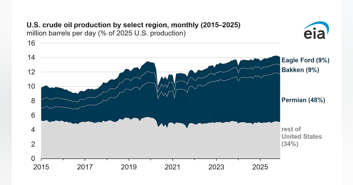
US crude output sets new record in 2025, Permian leads growth
Crude oil production in the US hit 13.6 million b/d in 2025, up 3% from the prior year, marking a new annual high, according to the US Energy Information Administration‘s (EIA) Short-Term Energy Outlook (STEO). Most of the increase came from the Lower 48 (excluding the Gulf of Mexico), which contributed 11.3 million b/d—roughly 83% of total production. Alaska and the US federal offshore Gulf of Mexico supplied the remainder. Production gains came despite a dip in drilling activity. Active rigs in the Lower 48 fell 5%, and completions slipped 1% versus 2024. Efficiency improvements kept output rising. New wells added 2.9 million b/d, while existing wells continued producing 8.3 million b/d. The slowdown reflected weaker prices, with WTI averaging $65/bbl, down from $77/bbl in 2024. The Permian basin remained the powerhouse of US production, accounting for 48% of total output at 6.6 million b/d and driving most of the year’s growth with a 280,000 b/d gain. Dallas Fed survey data show breakeven costs of $61–62/bbl in the Permian’s Midland and Delaware basins, supporting production even at lower prices. Elsewhere, output in the Eagle Ford and Bakken held mostly steady, each contributing about 9% of US crude. Eagle Ford edged up 18,000 b/d to 1.2 million b/d, while Bakken slipped 30,000 b/d to 1.2 million b/d. Five Gulf of Mexico projects supported 2025 production gains, combining new floating production units and subsea tiebacks. Output increased by 111,000 b/d to average 1.9 million b/d in 2025. The Shell plc-operated Whale development started production in January 2025. The deepwater development lies in more than 8,600 ft of water and is expected to produce about 85,000 b/d at peak. Shell’s Dover project came online in April as a tieback to the Appomattox hub, contributing 15,000 b/d. Also online in April was the Chevron-operated Ballymore project.

Greenland Energy secures rig for Arctic exploration
Greenland Energy Co. signed a drilling agreement with Stampede Drilling Inc. to provide a high-performance rig and services for upcoming operations in the Jameson Land basin. This agreement ensures the availability of Stampede’s Rig #12, equipped for Arctic conditions, to mobilize crews and execute drilling. Under a 5-year agreement, plans call for drilling up to two wells. Greenland Energy Co. was formed following completion of a deal to combine Pelican Holdco Inc., Pelican Acquisition Corp., March GL Co., and Greenland Exploration Ltd. According to 80 Mile PLC, Greenland Energy’s joint venture partner, the plan calls for each well to drill to a minimum depth of 3,500 m in an effort to delineate the hydrocarbon potential of the basin, which it said is analogous to the Norwegian Haltenbanken and Barents Sea provinces. Four petroleum systems have been identified with key source rocks – Upper Jurassic, Hareelv & Permian Ravnefjeld formations. Jameson comprises about two million acres in East Greenland. An independent prospective resources report prepared by Sproule ERCE estimated 13.03 billion bbl (P10) of gross un-risked recoverable prospective oil resources across the upper levels of the Jameson basin, 80 Mile PLC said in a February release. The partner also noted Greenland Energy has mobilized heavy equipment to East Greenland in preparation for drilling in this year’s second half, subject to regulatory approvals, and that Halliburton and IPT Well Solutions have been contracted to perform drilling services.
Chevron’s Aseng project advances with subsea infrastructure contract
@import url(‘https://fonts.googleapis.com/css2?family=Inter:[email protected]&display=swap’); a { color: var(–color-primary-main); } .ebm-page__main h1, .ebm-page__main h2, .ebm-page__main h3, .ebm-page__main h4, .ebm-page__main h5, .ebm-page__main h6 { font-family: Inter; } body { line-height: 150%; letter-spacing: 0.025em; font-family: Inter; } button, .ebm-button-wrapper { font-family: Inter; } .label-style { text-transform: uppercase; color: var(–color-grey); font-weight: 600; font-size: 0.75rem; } .caption-style { font-size: 0.75rem; opacity: .6; } #onetrust-pc-sdk [id*=btn-handler], #onetrust-pc-sdk [class*=btn-handler] { background-color: #c19a06 !important; border-color: #c19a06 !important; } #onetrust-policy a, #onetrust-pc-sdk a, #ot-pc-content a { color: #c19a06 !important; } #onetrust-consent-sdk #onetrust-pc-sdk .ot-active-menu { border-color: #c19a06 !important; } #onetrust-consent-sdk #onetrust-accept-btn-handler, #onetrust-banner-sdk #onetrust-reject-all-handler, #onetrust-consent-sdk #onetrust-pc-btn-handler.cookie-setting-link { background-color: #c19a06 !important; border-color: #c19a06 !important; } #onetrust-consent-sdk .onetrust-pc-btn-handler { color: #c19a06 !important; border-color: #c19a06 !important; } Noble Energy EG Ltd., a Chevron Corp. company, has let a contract to Subsea 7 for the subsea installation scope on the Aseng Gas Monetization Project offshore Equatorial Guinea. The work covers the transport and installation of about 19 km of rigid production flowline and 20 km of umbilicals, along with associated subsea structures and tie-ins in water depths of 800 m. Project management and engineering will begin immediately and will be managed from Subsea7’s Paris office, with additional support from teams in Lisbon and Equatorial Guinea. Offshore activities are expected to begin this year. Gas volumes from Aseng are expected to underpin the technical and commercial viability of multiple downstream and upstream developments under the Extended Gas Mega Hub initiative, including the Alen Tail, Yoyo-Yolanda, new drilling in Chevron-operated blocks, and potential cross-border gas flows through Gulf of Guinea pipeline infrastructure.

Oil prices surge as Iran war escalates, IEA warns of historic supply shock
Global oil markets rallied sharply on Thursday, Apr. 2, after US President Donald Trump signaled that military operations against Iran would continue “well into April,” raising fears of prolonged disruption to one of the world’s most critical energy corridors and triggering a fresh wave of volatility across commodities and financial markets. The renewed advance came just one day after markets had briefly turned more optimistic on hopes that the war might wind down soon. But Trump’s tougher tone shifted sentiment quickly, with investors focusing again on the Strait of Hormuz, the critical waterway that normally carries about one-fifth of the world’s oil and LNG trade. With traffic through the strait still heavily disrupted, the market remains highly sensitive to any sign that the conflict could drag on. Brent crude climbed toward $110/bbl in early trading, reversing earlier losses, as investors rapidly repriced geopolitical risk following Trump’s remarks that US forces would “finish the job” in Iran. Looming energy supply shock The latest market move also comes as the International Energy Agency (IEA) warns the unfolding crisis could evolve into the largest energy supply shock in modern history. Speaking this week, IEA Executive Director Fatih Birol said disruptions tied to the conflict are already mounting and could intensify significantly in April, with Europe among the most exposed regions. “The next month, April, will be much worse than March,” Birol said in an interview with Nicolai Tangen, chief executive officer of Norway’s Norges Bank Investment Management, on Tangen’s “In Good Company” podcast. The reason, Birol explained, is simple logistics. A trickle of cargo ships that entered the Strait before the US-Israel strikes on Iran have been continuing to deliver oil and gas to ports throughout March. “They are still coming to ports, still bringing oil and energy and other things,” he said.

Oil, gas industry secures Endangered Species Act exemption in Gulf of Mexico
The oil and gas industry has been granted an exemption from certain requirements under the Endangered Species Act (ESA) after a little-known commission, last convened in 1992, voted Mar. 31 on a matter covering federal oil and gas activities in the US Gulf of Mexico, citing national security concerns. The Endangered Species Committee voted unanimously to allow the exemption, which could make it more difficult for conservation and environmental groups to challenge projects under the ESA and protect endangered species such as the Rice’s whale. The committee is composed of the Secretaries of Interior, Agriculture and the Army, and the heads of the Council of Economic Advisers, Environmental Protection Agency, and National Oceanic and Atmospheric Administration. The meeting, which was live-streamed and lasted about 15 minutes, was convened after the Defense Secretary determined that an exemption was necessary for national security. “This meeting made clear that energy streams in the Gulf of America must not be disrupted or held hostage by ongoing litigation,” said Interior Secretary Doug Burgum in a press release. He said energy production in the Gulf “is indispensable to our nation’s strength, safeguarding our energy independence and preventing reliance on foreign adversaries,” and that “robust development in the Gulf keeps our economy resilient, stabilizes costs for American families and secures the US as a global leader for decades to come.” The exemption would apply to all federal oil and gas exploration, development, and production activities associated with the Bureau of Ocean Energy Management and BSEE Outer Continental Shelf oil and gas program. The Center for Biological Diversity had filed an emergency lawsuit in mid-March to prevent the Endangered Species Committee from conducting the meeting aimed at overriding a May 2025 National Marine Fisheries Service opinion that required mitigation measures such as vessel speed restrictions and monitoring to reduce

EIA: US oil inventories increase by 5.5 million bbl
US crude oil inventories, excluding those in the Strategic Petroleum Reserve, increased by 5.5 million bbl during the week ended Mar. 27 compared with the previous week’s total, according to the US Energy Information Administration’s (EIA) Petroleum Status Report. At 461.6 million bbl, US crude inventories are about 0.1% above the 5-year average. Total motor gasoline inventories decreased 600,000 bbl last week but are about 4% above the 5-year average. Finished gasoline inventories increased while blending components inventories decreased. Distillate fuel inventories decreased by 2.1 million bbl and are about 3% below the 5-year average for this time of year. Propane-propylene inventories increased by 4.1 million bbl from last week and are 71% above the 5-year average. Total commercial petroleum inventories decreased by 2.1 million bbl. US crude refinery inputs during the week averaged 16.4 million b/d, down 220,000 b/d from the previous week’s average. Refineries operated at 92.1% of their operable capacity. Gasoline production decreased, averaging 9.6 million b/d. Distillate fuel production remained steady, averaging 5.0 million b/d. US crude imports averaged 6.5 million b/d, down 10,000 b/d from the previous week’s average. Over the last 4 weeks, crude imports averaged 6.6 million b/d, up 12.8% from the same 4-week period last year. Total motor gasoline imports, including both finished gasoline and gasoline blending components, averaged 502,000 b/d. Distillate fuel imports averaged 117,000 b/d last week.
US crude output sets new record in 2025, Permian leads growth
Crude oil production in the US hit 13.6 million b/d in 2025, up 3% from the prior year, marking a new annual high, according to the US Energy Information Administration‘s (EIA) Short-Term Energy Outlook (STEO). Most of the increase came from the Lower 48 (excluding the Gulf of Mexico), which contributed 11.3 million b/d—roughly 83% of total production. Alaska and the US federal offshore Gulf of Mexico supplied the remainder. Production gains came despite a dip in drilling activity. Active rigs in the Lower 48 fell 5%, and completions slipped 1% versus 2024. Efficiency improvements kept output rising. New wells added 2.9 million b/d, while existing wells continued producing 8.3 million b/d. The slowdown reflected weaker prices, with WTI averaging $65/bbl, down from $77/bbl in 2024. The Permian basin remained the powerhouse of US production, accounting for 48% of total output at 6.6 million b/d and driving most of the year’s growth with a 280,000 b/d gain. Dallas Fed survey data show breakeven costs of $61–62/bbl in the Permian’s Midland and Delaware basins, supporting production even at lower prices. Elsewhere, output in the Eagle Ford and Bakken held mostly steady, each contributing about 9% of US crude. Eagle Ford edged up 18,000 b/d to 1.2 million b/d, while Bakken slipped 30,000 b/d to 1.2 million b/d. Five Gulf of Mexico projects supported 2025 production gains, combining new floating production units and subsea tiebacks. Output increased by 111,000 b/d to average 1.9 million b/d in 2025. The Shell plc-operated Whale development started production in January 2025. The deepwater development lies in more than 8,600 ft of water and is expected to produce about 85,000 b/d at peak. Shell’s Dover project came online in April as a tieback to the Appomattox hub, contributing 15,000 b/d. Also online in April was the Chevron-operated Ballymore project.
Greenland Energy secures rig for Arctic exploration
Greenland Energy Co. signed a drilling agreement with Stampede Drilling Inc. to provide a high-performance rig and services for upcoming operations in the Jameson Land basin. This agreement ensures the availability of Stampede’s Rig #12, equipped for Arctic conditions, to mobilize crews and execute drilling. Under a 5-year agreement, plans call for drilling up to two wells. Greenland Energy Co. was formed following completion of a deal to combine Pelican Holdco Inc., Pelican Acquisition Corp., March GL Co., and Greenland Exploration Ltd. According to 80 Mile PLC, Greenland Energy’s joint venture partner, the plan calls for each well to drill to a minimum depth of 3,500 m in an effort to delineate the hydrocarbon potential of the basin, which it said is analogous to the Norwegian Haltenbanken and Barents Sea provinces. Four petroleum systems have been identified with key source rocks – Upper Jurassic, Hareelv & Permian Ravnefjeld formations. Jameson comprises about two million acres in East Greenland. An independent prospective resources report prepared by Sproule ERCE estimated 13.03 billion bbl (P10) of gross un-risked recoverable prospective oil resources across the upper levels of the Jameson basin, 80 Mile PLC said in a February release. The partner also noted Greenland Energy has mobilized heavy equipment to East Greenland in preparation for drilling in this year’s second half, subject to regulatory approvals, and that Halliburton and IPT Well Solutions have been contracted to perform drilling services.
Chevron’s Aseng project advances with subsea infrastructure contract
@import url(‘https://fonts.googleapis.com/css2?family=Inter:[email protected]&display=swap’); a { color: var(–color-primary-main); } .ebm-page__main h1, .ebm-page__main h2, .ebm-page__main h3, .ebm-page__main h4, .ebm-page__main h5, .ebm-page__main h6 { font-family: Inter; } body { line-height: 150%; letter-spacing: 0.025em; font-family: Inter; } button, .ebm-button-wrapper { font-family: Inter; } .label-style { text-transform: uppercase; color: var(–color-grey); font-weight: 600; font-size: 0.75rem; } .caption-style { font-size: 0.75rem; opacity: .6; } #onetrust-pc-sdk [id*=btn-handler], #onetrust-pc-sdk [class*=btn-handler] { background-color: #c19a06 !important; border-color: #c19a06 !important; } #onetrust-policy a, #onetrust-pc-sdk a, #ot-pc-content a { color: #c19a06 !important; } #onetrust-consent-sdk #onetrust-pc-sdk .ot-active-menu { border-color: #c19a06 !important; } #onetrust-consent-sdk #onetrust-accept-btn-handler, #onetrust-banner-sdk #onetrust-reject-all-handler, #onetrust-consent-sdk #onetrust-pc-btn-handler.cookie-setting-link { background-color: #c19a06 !important; border-color: #c19a06 !important; } #onetrust-consent-sdk .onetrust-pc-btn-handler { color: #c19a06 !important; border-color: #c19a06 !important; } Noble Energy EG Ltd., a Chevron Corp. company, has let a contract to Subsea 7 for the subsea installation scope on the Aseng Gas Monetization Project offshore Equatorial Guinea. The work covers the transport and installation of about 19 km of rigid production flowline and 20 km of umbilicals, along with associated subsea structures and tie-ins in water depths of 800 m. Project management and engineering will begin immediately and will be managed from Subsea7’s Paris office, with additional support from teams in Lisbon and Equatorial Guinea. Offshore activities are expected to begin this year. Gas volumes from Aseng are expected to underpin the technical and commercial viability of multiple downstream and upstream developments under the Extended Gas Mega Hub initiative, including the Alen Tail, Yoyo-Yolanda, new drilling in Chevron-operated blocks, and potential cross-border gas flows through Gulf of Guinea pipeline infrastructure.
Oil prices surge as Iran war escalates, IEA warns of historic supply shock
Global oil markets rallied sharply on Thursday, Apr. 2, after US President Donald Trump signaled that military operations against Iran would continue “well into April,” raising fears of prolonged disruption to one of the world’s most critical energy corridors and triggering a fresh wave of volatility across commodities and financial markets. The renewed advance came just one day after markets had briefly turned more optimistic on hopes that the war might wind down soon. But Trump’s tougher tone shifted sentiment quickly, with investors focusing again on the Strait of Hormuz, the critical waterway that normally carries about one-fifth of the world’s oil and LNG trade. With traffic through the strait still heavily disrupted, the market remains highly sensitive to any sign that the conflict could drag on. Brent crude climbed toward $110/bbl in early trading, reversing earlier losses, as investors rapidly repriced geopolitical risk following Trump’s remarks that US forces would “finish the job” in Iran. Looming energy supply shock The latest market move also comes as the International Energy Agency (IEA) warns the unfolding crisis could evolve into the largest energy supply shock in modern history. Speaking this week, IEA Executive Director Fatih Birol said disruptions tied to the conflict are already mounting and could intensify significantly in April, with Europe among the most exposed regions. “The next month, April, will be much worse than March,” Birol said in an interview with Nicolai Tangen, chief executive officer of Norway’s Norges Bank Investment Management, on Tangen’s “In Good Company” podcast. The reason, Birol explained, is simple logistics. A trickle of cargo ships that entered the Strait before the US-Israel strikes on Iran have been continuing to deliver oil and gas to ports throughout March. “They are still coming to ports, still bringing oil and energy and other things,” he said.
Oil, gas industry secures Endangered Species Act exemption in Gulf of Mexico
The oil and gas industry has been granted an exemption from certain requirements under the Endangered Species Act (ESA) after a little-known commission, last convened in 1992, voted Mar. 31 on a matter covering federal oil and gas activities in the US Gulf of Mexico, citing national security concerns. The Endangered Species Committee voted unanimously to allow the exemption, which could make it more difficult for conservation and environmental groups to challenge projects under the ESA and protect endangered species such as the Rice’s whale. The committee is composed of the Secretaries of Interior, Agriculture and the Army, and the heads of the Council of Economic Advisers, Environmental Protection Agency, and National Oceanic and Atmospheric Administration. The meeting, which was live-streamed and lasted about 15 minutes, was convened after the Defense Secretary determined that an exemption was necessary for national security. “This meeting made clear that energy streams in the Gulf of America must not be disrupted or held hostage by ongoing litigation,” said Interior Secretary Doug Burgum in a press release. He said energy production in the Gulf “is indispensable to our nation’s strength, safeguarding our energy independence and preventing reliance on foreign adversaries,” and that “robust development in the Gulf keeps our economy resilient, stabilizes costs for American families and secures the US as a global leader for decades to come.” The exemption would apply to all federal oil and gas exploration, development, and production activities associated with the Bureau of Ocean Energy Management and BSEE Outer Continental Shelf oil and gas program. The Center for Biological Diversity had filed an emergency lawsuit in mid-March to prevent the Endangered Species Committee from conducting the meeting aimed at overriding a May 2025 National Marine Fisheries Service opinion that required mitigation measures such as vessel speed restrictions and monitoring to reduce
EIA: US oil inventories increase by 5.5 million bbl
US crude oil inventories, excluding those in the Strategic Petroleum Reserve, increased by 5.5 million bbl during the week ended Mar. 27 compared with the previous week’s total, according to the US Energy Information Administration’s (EIA) Petroleum Status Report. At 461.6 million bbl, US crude inventories are about 0.1% above the 5-year average. Total motor gasoline inventories decreased 600,000 bbl last week but are about 4% above the 5-year average. Finished gasoline inventories increased while blending components inventories decreased. Distillate fuel inventories decreased by 2.1 million bbl and are about 3% below the 5-year average for this time of year. Propane-propylene inventories increased by 4.1 million bbl from last week and are 71% above the 5-year average. Total commercial petroleum inventories decreased by 2.1 million bbl. US crude refinery inputs during the week averaged 16.4 million b/d, down 220,000 b/d from the previous week’s average. Refineries operated at 92.1% of their operable capacity. Gasoline production decreased, averaging 9.6 million b/d. Distillate fuel production remained steady, averaging 5.0 million b/d. US crude imports averaged 6.5 million b/d, down 10,000 b/d from the previous week’s average. Over the last 4 weeks, crude imports averaged 6.6 million b/d, up 12.8% from the same 4-week period last year. Total motor gasoline imports, including both finished gasoline and gasoline blending components, averaged 502,000 b/d. Distillate fuel imports averaged 117,000 b/d last week.
Chevron’s Aseng project advances with subsea infrastructure contract
@import url(‘https://fonts.googleapis.com/css2?family=Inter:[email protected]&display=swap’); a { color: var(–color-primary-main); } .ebm-page__main h1, .ebm-page__main h2, .ebm-page__main h3, .ebm-page__main h4, .ebm-page__main h5, .ebm-page__main h6 { font-family: Inter; } body { line-height: 150%; letter-spacing: 0.025em; font-family: Inter; } button, .ebm-button-wrapper { font-family: Inter; } .label-style { text-transform: uppercase; color: var(–color-grey); font-weight: 600; font-size: 0.75rem; } .caption-style { font-size: 0.75rem; opacity: .6; } #onetrust-pc-sdk [id*=btn-handler], #onetrust-pc-sdk [class*=btn-handler] { background-color: #c19a06 !important; border-color: #c19a06 !important; } #onetrust-policy a, #onetrust-pc-sdk a, #ot-pc-content a { color: #c19a06 !important; } #onetrust-consent-sdk #onetrust-pc-sdk .ot-active-menu { border-color: #c19a06 !important; } #onetrust-consent-sdk #onetrust-accept-btn-handler, #onetrust-banner-sdk #onetrust-reject-all-handler, #onetrust-consent-sdk #onetrust-pc-btn-handler.cookie-setting-link { background-color: #c19a06 !important; border-color: #c19a06 !important; } #onetrust-consent-sdk .onetrust-pc-btn-handler { color: #c19a06 !important; border-color: #c19a06 !important; } Noble Energy EG Ltd., a Chevron Corp. company, has let a contract to Subsea 7 for the subsea installation scope on the Aseng Gas Monetization Project offshore Equatorial Guinea. The work covers the transport and installation of about 19 km of rigid production flowline and 20 km of umbilicals, along with associated subsea structures and tie-ins in water depths of 800 m. Project management and engineering will begin immediately and will be managed from Subsea7’s Paris office, with additional support from teams in Lisbon and Equatorial Guinea. Offshore activities are expected to begin this year. Gas volumes from Aseng are expected to underpin the technical and commercial viability of multiple downstream and upstream developments under the Extended Gas Mega Hub initiative, including the Alen Tail, Yoyo-Yolanda, new drilling in Chevron-operated blocks, and potential cross-border gas flows through Gulf of Guinea pipeline infrastructure.
Greenland Energy secures rig for Arctic exploration
Greenland Energy Co. signed a drilling agreement with Stampede Drilling Inc. to provide a high-performance rig and services for upcoming operations in the Jameson Land basin. This agreement ensures the availability of Stampede’s Rig #12, equipped for Arctic conditions, to mobilize crews and execute drilling. Under a 5-year agreement, plans call for drilling up to two wells. Greenland Energy Co. was formed following completion of a deal to combine Pelican Holdco Inc., Pelican Acquisition Corp., March GL Co., and Greenland Exploration Ltd. According to 80 Mile PLC, Greenland Energy’s joint venture partner, the plan calls for each well to drill to a minimum depth of 3,500 m in an effort to delineate the hydrocarbon potential of the basin, which it said is analogous to the Norwegian Haltenbanken and Barents Sea provinces. Four petroleum systems have been identified with key source rocks – Upper Jurassic, Hareelv & Permian Ravnefjeld formations. Jameson comprises about two million acres in East Greenland. An independent prospective resources report prepared by Sproule ERCE estimated 13.03 billion bbl (P10) of gross un-risked recoverable prospective oil resources across the upper levels of the Jameson basin, 80 Mile PLC said in a February release. The partner also noted Greenland Energy has mobilized heavy equipment to East Greenland in preparation for drilling in this year’s second half, subject to regulatory approvals, and that Halliburton and IPT Well Solutions have been contracted to perform drilling services.
US crude output sets new record in 2025, Permian leads growth
Crude oil production in the US hit 13.6 million b/d in 2025, up 3% from the prior year, marking a new annual high, according to the US Energy Information Administration‘s (EIA) Short-Term Energy Outlook (STEO). Most of the increase came from the Lower 48 (excluding the Gulf of Mexico), which contributed 11.3 million b/d—roughly 83% of total production. Alaska and the US federal offshore Gulf of Mexico supplied the remainder. Production gains came despite a dip in drilling activity. Active rigs in the Lower 48 fell 5%, and completions slipped 1% versus 2024. Efficiency improvements kept output rising. New wells added 2.9 million b/d, while existing wells continued producing 8.3 million b/d. The slowdown reflected weaker prices, with WTI averaging $65/bbl, down from $77/bbl in 2024. The Permian basin remained the powerhouse of US production, accounting for 48% of total output at 6.6 million b/d and driving most of the year’s growth with a 280,000 b/d gain. Dallas Fed survey data show breakeven costs of $61–62/bbl in the Permian’s Midland and Delaware basins, supporting production even at lower prices. Elsewhere, output in the Eagle Ford and Bakken held mostly steady, each contributing about 9% of US crude. Eagle Ford edged up 18,000 b/d to 1.2 million b/d, while Bakken slipped 30,000 b/d to 1.2 million b/d. Five Gulf of Mexico projects supported 2025 production gains, combining new floating production units and subsea tiebacks. Output increased by 111,000 b/d to average 1.9 million b/d in 2025. The Shell plc-operated Whale development started production in January 2025. The deepwater development lies in more than 8,600 ft of water and is expected to produce about 85,000 b/d at peak. Shell’s Dover project came online in April as a tieback to the Appomattox hub, contributing 15,000 b/d. Also online in April was the Chevron-operated Ballymore project.

QatarEnergy, ExxonMobil reach first production from Train 1 at Golden Pass
@import url(‘https://fonts.googleapis.com/css2?family=Inter:[email protected]&display=swap’); a { color: var(–color-primary-main); } .ebm-page__main h1, .ebm-page__main h2, .ebm-page__main h3, .ebm-page__main h4, .ebm-page__main h5, .ebm-page__main h6 { font-family: Inter; } body { line-height: 150%; letter-spacing: 0.025em; font-family: Inter; } button, .ebm-button-wrapper { font-family: Inter; } .label-style { text-transform: uppercase; color: var(–color-grey); font-weight: 600; font-size: 0.75rem; } .caption-style { font-size: 0.75rem; opacity: .6; } #onetrust-pc-sdk [id*=btn-handler], #onetrust-pc-sdk [class*=btn-handler] { background-color: #c19a06 !important; border-color: #c19a06 !important; } #onetrust-policy a, #onetrust-pc-sdk a, #ot-pc-content a { color: #c19a06 !important; } #onetrust-consent-sdk #onetrust-pc-sdk .ot-active-menu { border-color: #c19a06 !important; } #onetrust-consent-sdk #onetrust-accept-btn-handler, #onetrust-banner-sdk #onetrust-reject-all-handler, #onetrust-consent-sdk #onetrust-pc-btn-handler.cookie-setting-link { background-color: #c19a06 !important; border-color: #c19a06 !important; } #onetrust-consent-sdk .onetrust-pc-btn-handler { color: #c19a06 !important; border-color: #c19a06 !important; } Golden Pass LNG, a joint venture between QatarEnergy and ExxonMobil, reached first production of LNG from Train 1 at the export project in Sabine Pass, Tex. With first LNG completed, the joint venture advances work to deliver its first cargo, achieve sustained liquefaction operations, and meet its commercial and strategic objectives, ExxonMobil said in a release Mar. 30. Train 1 is one of three LNG trains comprising the 18-million tonnes/year plant. The start of LNG exports to global customers is expected in this year’s second quarter. QatarEnergy holds 70% interest in Golden Pass LNG, while ExxonMobil holds the remaining 30%.

Chevron resumes natural gas production at Leviathan
@import url(‘https://fonts.googleapis.com/css2?family=Inter:[email protected]&display=swap’); a { color: var(–color-primary-main); } .ebm-page__main h1, .ebm-page__main h2, .ebm-page__main h3, .ebm-page__main h4, .ebm-page__main h5, .ebm-page__main h6 { font-family: Inter; } body { line-height: 150%; letter-spacing: 0.025em; font-family: Inter; } button, .ebm-button-wrapper { font-family: Inter; } .label-style { text-transform: uppercase; color: var(–color-grey); font-weight: 600; font-size: 0.75rem; } .caption-style { font-size: 0.75rem; opacity: .6; } #onetrust-pc-sdk [id*=btn-handler], #onetrust-pc-sdk [class*=btn-handler] { background-color: #c19a06 !important; border-color: #c19a06 !important; } #onetrust-policy a, #onetrust-pc-sdk a, #ot-pc-content a { color: #c19a06 !important; } #onetrust-consent-sdk #onetrust-pc-sdk .ot-active-menu { border-color: #c19a06 !important; } #onetrust-consent-sdk #onetrust-accept-btn-handler, #onetrust-banner-sdk #onetrust-reject-all-handler, #onetrust-consent-sdk #onetrust-pc-btn-handler.cookie-setting-link { background-color: #c19a06 !important; border-color: #c19a06 !important; } #onetrust-consent-sdk .onetrust-pc-btn-handler { color: #c19a06 !important; border-color: #c19a06 !important; } Chevron Mediterranean Ltd. restarted production at the Leviathan natural gas field 130 km offshore Haifa in the eastern Mediterranean after a suspension due to the Iran war, partner NewMed Energy said in a release. The operator had previously received clearance from the Petroleum Commissioner to proceed with preparations to resume operations at the Leviathan platform offshore Israel. Regular production from the reservoir was restarted on Apr. 2. Chevron is operator at Leviathan (39.66%) with partners NewMed Energy (45.34%) and Ratio Energies (15%).

Energy Department Authorizes Additional Exports of LNG from Elba Island Terminal, Strengthening Global Energy Supply with U.S. LNG
WASHINGTON—U.S. Secretary of Energy Chris Wright today authorized an immediate 22% increase in exports of liquefied natural gas (LNG) from the Elba Island Terminal in Chatham County, Georgia. With today’s order, Kinder Morgan subsidiary Southern LNG Company L.L.C., operator of the Elba Island LNG Terminal, is now authorized to export up to an additional 28.25 (Bcf/yr) to non-free trade agreement countries, strengthening global natural gas supplies with reliable U.S. LNG. Elba Island was previously authorized to export up to 130 billion cubic feet per year (Bcf/yr) of natural gas as LNG to non-free trade agreement countries and has been exporting U.S. LNG since 2019. The project is positioned to export the additional approved volumes immediately. “At a time when global energy supply routes face disruption, the United States remains a reliable energy partner to our allies and trading partners,” said DOE Assistant Secretary of the Hydrocarbons and Geothermal Energy Office, Kyle Haustveit. “DOE is using all available authorities to ensure American energy can reach global markets when it is needed most, supporting energy security and helping stabilize global energy supplies.” The action comes as global oil and LNG supply routes face disruption from tensions in the Middle East and attacks carried out by Iran and its proxies, threatening the reliable flow of energy through critical maritime corridors. The Department will continue to act, using its full set of authorities, to ensure U.S. LNG remains a dependable energy source in global energy markets and a stabilizing presence in times of disruption. Thanks to President Trump’s leadership and American innovation, the United States is the world’s largest natural gas producer and exporter, with exports reaching all-time highs in March 2026. Since President Trump ended the previous administration’s LNG export approval ban, the Department has approved more than 19 Bcf/d of LNG export authorizations. With recent final investment decisions for additional export capacity, U.S. LNG exports are set

National Grid, Con Edison urge FERC to adopt gas pipeline reliability requirements
The Federal Energy Regulatory Commission should adopt reliability-related requirements for gas pipeline operators to ensure fuel supplies during cold weather, according to National Grid USA and affiliated utilities Consolidated Edison Co. of New York and Orange and Rockland Utilities. In the wake of power outages in the Southeast and the near collapse of New York City’s gas system during Winter Storm Elliott in December 2022, voluntary efforts to bolster gas pipeline reliability are inadequate, the utilities said in two separate filings on Friday at FERC. The filings were in response to a gas-electric coordination meeting held in November by the Federal-State Current Issues Collaborative between FERC and the National Association of Regulatory Utility Commissioners. National Grid called for FERC to use its authority under the Natural Gas Act to require pipeline reliability reporting, coupled with enforcement mechanisms, and pipeline tariff reforms. “Such data reporting would enable the commission to gain a clearer picture into pipeline reliability and identify any problematic trends in the quality of pipeline service,” National Grid said. “At that point, the commission could consider using its ratemaking, audit, and civil penalty authority preemptively to address such identified concerns before they result in service curtailments.” On pipeline tariff reforms, FERC should develop tougher provisions for force majeure events — an unforeseen occurence that prevents a contract from being fulfilled — reservation charge crediting, operational flow orders, scheduling and confirmation enhancements, improved real-time coordination, and limits on changes to nomination rankings, National Grid said. FERC should support efforts in New England and New York to create financial incentives for gas-fired generators to enter into winter contracts for imported liquefied natural gas supplies, or other long-term firm contracts with suppliers and pipelines, National Grid said. Con Edison and O&R said they were encouraged by recent efforts such as North American Energy Standard

US BOEM Seeks Feedback on Potential Wind Leasing Offshore Guam
The United States Bureau of Ocean Energy Management (BOEM) on Monday issued a Call for Information and Nominations to help it decide on potential leasing areas for wind energy development offshore Guam. The call concerns a contiguous area around the island that comprises about 2.1 million acres. The area’s water depths range from 350 meters (1,148.29 feet) to 2,200 meters (7,217.85 feet), according to a statement on BOEM’s website. Closing April 7, the comment period seeks “relevant information on site conditions, marine resources, and ocean uses near or within the call area”, the BOEM said. “Concurrently, wind energy companies can nominate specific areas they would like to see offered for leasing. “During the call comment period, BOEM will engage with Indigenous Peoples, stakeholder organizations, ocean users, federal agencies, the government of Guam, and other parties to identify conflicts early in the process as BOEM seeks to identify areas where offshore wind development would have the least impact”. The next step would be the identification of specific WEAs, or wind energy areas, in the larger call area. BOEM would then conduct environmental reviews of the WEAs in consultation with different stakeholders. “After completing its environmental reviews and consultations, BOEM may propose one or more competitive lease sales for areas within the WEAs”, the Department of the Interior (DOI) sub-agency said. BOEM Director Elizabeth Klein said, “Responsible offshore wind development off Guam’s coast offers a vital opportunity to expand clean energy, cut carbon emissions, and reduce energy costs for Guam residents”. Late last year the DOI announced the approval of the 2.4-gigawatt (GW) SouthCoast Wind Project, raising the total capacity of federally approved offshore wind power projects to over 19 GW. The project owned by a joint venture between EDP Renewables and ENGIE received a positive Record of Decision, the DOI said in

Biden Bars Offshore Oil Drilling in USA Atlantic and Pacific
President Joe Biden is indefinitely blocking offshore oil and gas development in more than 625 million acres of US coastal waters, warning that drilling there is simply “not worth the risks” and “unnecessary” to meet the nation’s energy needs. Biden’s move is enshrined in a pair of presidential memoranda being issued Monday, burnishing his legacy on conservation and fighting climate change just two weeks before President-elect Donald Trump takes office. Yet unlike other actions Biden has taken to constrain fossil fuel development, this one could be harder for Trump to unwind, since it’s rooted in a 72-year-old provision of federal law that empowers presidents to withdraw US waters from oil and gas leasing without explicitly authorizing revocations. Biden is ruling out future oil and gas leasing along the US East and West Coasts, the eastern Gulf of Mexico and a sliver of the Northern Bering Sea, an area teeming with seabirds, marine mammals, fish and other wildlife that indigenous people have depended on for millennia. The action doesn’t affect energy development under existing offshore leases, and it won’t prevent the sale of more drilling rights in Alaska’s gas-rich Cook Inlet or the central and western Gulf of Mexico, which together provide about 14% of US oil and gas production. The president cast the move as achieving a careful balance between conservation and energy security. “It is clear to me that the relatively minimal fossil fuel potential in the areas I am withdrawing do not justify the environmental, public health and economic risks that would come from new leasing and drilling,” Biden said. “We do not need to choose between protecting the environment and growing our economy, or between keeping our ocean healthy, our coastlines resilient and the food they produce secure — and keeping energy prices low.” Some of the areas Biden is protecting

Biden Admin Finalizes Hydrogen Tax Credit Favoring Cleaner Production
The Biden administration has finalized rules for a tax incentive promoting hydrogen production using renewable power, with lower credits for processes using abated natural gas. The Clean Hydrogen Production Credit is based on carbon intensity, which must not exceed four kilograms of carbon dioxide equivalent per kilogram of hydrogen produced. Qualified facilities are those whose start of construction falls before 2033. These facilities can claim credits for 10 years of production starting on the date of service placement, according to the draft text on the Federal Register’s portal. The final text is scheduled for publication Friday. Established by the 2022 Inflation Reduction Act, the four-tier scheme gives producers that meet wage and apprenticeship requirements a credit of up to $3 per kilogram of “qualified clean hydrogen”, to be adjusted for inflation. Hydrogen whose production process makes higher lifecycle emissions gets less. The scheme will use the Energy Department’s Greenhouse Gases, Regulated Emissions and Energy Use in Transportation (GREET) model in tiering production processes for credit computation. “In the coming weeks, the Department of Energy will release an updated version of the 45VH2-GREET model that producers will use to calculate the section 45V tax credit”, the Treasury Department said in a statement announcing the finalization of rules, a process that it said had considered roughly 30,000 public comments. However, producers may use the GREET model that was the most recent when their facility began construction. “This is in consideration of comments that the prospect of potential changes to the model over time reduces investment certainty”, explained the statement on the Treasury’s website. “Calculation of the lifecycle GHG analysis for the tax credit requires consideration of direct and significant indirect emissions”, the statement said. For electrolytic hydrogen, electrolyzers covered by the scheme include not only those using renewables-derived electricity (green hydrogen) but

Xthings unveils Ulticam home security cameras powered by edge AI
Join our daily and weekly newsletters for the latest updates and exclusive content on industry-leading AI coverage. Learn More Xthings announced that its Ulticam security camera brand has a new model out today: the Ulticam IQ Floodlight, an edge AI-powered home security camera. The company also plans to showcase two additional cameras, Ulticam IQ, an outdoor spotlight camera, and Ulticam Dot, a portable, wireless security camera. All three cameras offer free cloud storage (seven days rolling) and subscription-free edge AI-powered person detection and alerts. The AI at the edge means that it doesn’t have to go out to an internet-connected data center to tap AI computing to figure out what is in front of the camera. Rather, the processing for the AI is built into the camera itself, and that sets a new standard for value and performance in home security cameras. It can identify people, faces and vehicles. CES 2025 attendees can experience Ulticam’s entire lineup at Pepcom’s Digital Experience event on January 6, 2025, and at the Venetian Expo, Halls A-D, booth #51732, from January 7 to January 10, 2025. These new security cameras will be available for purchase online in the U.S. in Q1 and Q2 2025 at U-tec.com, Amazon, and Best Buy. The Ulticam IQ Series: smart edge AI-powered home security cameras Ulticam IQ home security camera. The Ulticam IQ Series, which includes IQ and IQ Floodlight, takes home security to the next level with the most advanced AI-powered recognition. Among the very first consumer cameras to use edge AI, the IQ Series can quickly and accurately identify people, faces and vehicles, without uploading video for server-side processing, which improves speed, accuracy, security and privacy. Additionally, the Ulticam IQ Series is designed to improve over time with over-the-air updates that enable new AI features. Both cameras

Intel unveils new Core Ultra processors with 2X to 3X performance on AI apps
Join our daily and weekly newsletters for the latest updates and exclusive content on industry-leading AI coverage. Learn More Intel unveiled new Intel Core Ultra 9 processors today at CES 2025 with as much as two or three times the edge performance on AI apps as before. The chips under the Intel Core Ultra 9 and Core i9 labels were previously codenamed Arrow Lake H, Meteor Lake H, Arrow Lake S and Raptor Lake S Refresh. Intel said it is pushing the boundaries of AI performance and power efficiency for businesses and consumers, ushering in the next era of AI computing. In other performance metrics, Intel said the Core Ultra 9 processors are up to 5.8 times faster in media performance, 3.4 times faster in video analytics end-to-end workloads with media and AI, and 8.2 times better in terms of performance per watt than prior chips. Intel hopes to kick off the year better than in 2024. CEO Pat Gelsinger resigned last month without a permanent successor after a variety of struggles, including mass layoffs, manufacturing delays and poor execution on chips including gaming bugs in chips launched during the summer. Intel Core Ultra Series 2 Michael Masci, vice president of product management at the Edge Computing Group at Intel, said in a briefing that AI, once the domain of research labs, is integrating into every aspect of our lives, including AI PCs where the AI processing is done in the computer itself, not the cloud. AI is also being processed in data centers in big enterprises, from retail stores to hospital rooms. “As CES kicks off, it’s clear we are witnessing a transformative moment,” he said. “Artificial intelligence is moving at an unprecedented pace.” The new processors include the Intel Core 9 Ultra 200 H/U/S models, with up to
Shifting to AI model customization is an architectural imperative
In partnership withMistral AI In the early days of large language models (LLMs), we grew accustomed to massive 10x jumps in reasoning and coding capability with every new model iteration. Today, those jumps have flattened into incremental gains. The exception is domain-specialized intelligence, where true step-function improvements are still the norm. When a model is fused with an organization’s proprietary data and internal logic, it encodes the company’s history into its future workflows. This alignment creates a compounding advantage: a competitive moat built on a model that understands the business intimately. This is more than fine-tuning; it is the institutionalization of expertise into an AI system. This is the power of customization. Intelligence tuned to context Every sector operates within its own specific lexicon. In automotive engineering, the “language” of the firm revolves around tolerance stacks, validation cycles, and revision control. In capital markets, reasoning is dictated by risk-weighted assets and liquidity buffers. In security operations, patterns are extracted from the noise of telemetry signals and identity anomalies. Custom-adapted models internalize the nuances of the field. They recognize which variables dictate a “go/no-go” decision, and they think in the language of the industry.
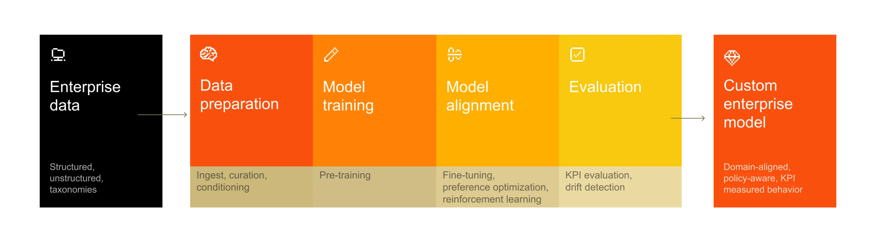
Domain expertise in action The transition from general-purpose to tailored AI centers on one goal: encoding an organization’s unique logic directly into a model’s weights. Mistral AI partners with organizations to incorporate domain expertise into their training ecosystems. A few use cases illustrate customized implementations in practice:
Software engineering and assisting at scale: A network hardware company with proprietary languages and specialized codebases found that out-of-the-box models could not grasp their internal stack. By training a custom model on their own development patterns, they achieved a step function in fluency. Integrated into Mistral’s software development scaffolding, this customized model now supports the entire lifecycle—from maintaining legacy systems to autonomous code modernization via reinforcement learning. This turns once-opaque, niche code into a space where AI reliably assists at scale. Automotive and the engineering copilot: A leading automotive company uses customization to revolutionize crash test simulations. Previously, specialists spent entire days manually comparing digital simulations with physical results to find divergences. By training a model on proprietary simulation data and internal analyses, they automated this visual inspection, flagging deformations in real time. Moving beyond detection, the model now acts as a copilot, proposing design adjustments to bring simulations closer to real-world behavior and radically accelerating the R&D loop. Public sector and sovereign AI: In Southeast Asia, a government agency is building a sovereign AI layer to move beyond Western-centric models. By commissioning a foundation model tailored to regional languages, local idioms, and cultural contexts, they created a strategic infrastructure asset. This ensures sensitive data remains under local governance while powering inclusive citizen services and regulatory assistants. Here, customization is the key to deploying AI that is both technically effective and genuinely sovereign. The blueprint for strategic customization Moving from a general-purpose AI strategy to a domain-specific advantage requires a structural rethinking of the model’s role within the enterprise. Success is defined by three shifts in organizational logic. 1. Treat AI as infrastructure, not an experiment. Historically, enterprises have treated model customization as an ad hoc experiment—a single fine-tuning run for a niche use case or a localized pilot. While these bespoke silos often yield promising results, they are rarely built to scale. They produce brittle pipelines, improvised governance, and limited portability. When the underlying base models evolve, the adaptation work must often be discarded and rebuilt from scratch.In contrast, a durable strategy treats customization as foundational infrastructure. In this model, adaptation workflows are reproducible, version-controlled, and engineered for production. Success is measured against deterministic business outcomes. By decoupling the customization logic from the underlying model, firms ensure that their “digital nervous system” remains resilient, even as the frontier of base models shifts. 2. Retain control of your own data and models. As AI migrates from the periphery to core operations, the question of control becomes existential. Reliance on a single cloud provider or vendor for model alignment creates a dangerous asymmetry of power regarding data residency, pricing, and architectural updates. Enterprises that retain control of their training pipelines and deployment environments preserve their strategic agency. By adapting models within controlled environments, organizations can enforce their own data residency requirements and dictate their own update cycles. This approach transforms AI from a service consumed into an asset governed, reducing structural dependency and allowing for cost and energy optimizations aligned with internal priorities rather than vendor roadmaps. 3. Design for continuous adaptation. The enterprise environment is never static: regulations shift, taxonomies evolve, and market conditions fluctuate. A common failure is treating a customized model as a finished artifact. In reality, a domain-aligned model is a living asset subject to model decay if left unmanaged.
Designing for continuous adaptation requires a disciplined approach to ModelOps. This includes automated drift detection, event-driven retraining, and incremental updates. By building the capacity for constant recalibration, the organization ensures that its AI does not just reflect its history, but it evolves in lockstep with its future. This is the stage where the competitive moat begins to compound: the model’s utility grows as it internalizes the organization’s ongoing response to change. Control is the new leverage We have entered an era where generic intelligence is a commodity, but contextual intelligence is a scarcity. While raw model power is now a baseline requirement, the true differentiator is alignment—AI calibrated to an organization’s unique data, mandates, and decision logic. In the next decade, the most valuable AI won’t be the one that knows everything about the world; it will be the one that knows everything about you. The firms that own the model weights of that intelligence will own the market. This content was produced by Mistral AI. It was not written by MIT Technology Review’s editorial staff.

AI benchmarks are broken. Here’s what we need instead.
For decades, artificial intelligence has been evaluated through the question of whether machines outperform humans. From chess to advanced math, from coding to essay writing, the performance of AI models and applications is tested against that of individual humans completing tasks. This framing is seductive: An AI vs. human comparison on isolated problems with clear right or wrong answers is easy to standardize, compare, and optimize. It generates rankings and headlines. But there’s a problem: AI is almost never used in the way it is benchmarked. Although researchers and industry have started to improve benchmarking by moving beyond static tests to more dynamic evaluation methods, these innovations resolve only part of the issue. That’s because they still evaluate AI’s performance outside the human teams and organizational workflows where its real-world performance ultimately unfolds. While AI is evaluated at the task level in a vacuum, it is used in messy, complex environments where it usually interacts with more than one person. Its performance (or lack thereof) emerges only over extended periods of use. This misalignment leaves us misunderstanding AI’s capabilities, overlooking systemic risks, and misjudging its economic and social consequences.
To mitigate this, it’s time to shift from narrow methods to benchmarks that assess how AI systems perform over longer time horizons within human teams, workflows, and organizations. I have studied real-world AI deployment since 2022 in small businesses and health, humanitarian, nonprofit, and higher-education organizations in the UK, the United States, and Asia, as well as within leading AI design ecosystems in London and Silicon Valley. I propose a different approach, which I call HAIC benchmarks—Human–AI, Context-Specific Evaluation. What happens when AI fails For governments and businesses, AI benchmark scores appear more objective than vendor claims. They’re a critical part of determining whether an AI model or application is “good enough” for real-world deployment. Imagine an AI model that achieves impressive technical scores on the most cutting-edge benchmarks—98% accuracy, groundbreaking speed, compelling outputs. On the strength of these results, organizations may decide to adopt the model, committing sizable financial and technical resources to purchasing and integrating it.
But then, once it’s adopted, the gap between benchmark and real-world performance quickly becomes visible. For example, take the swathe of FDA-approved AI models that can read medical scans faster and more accurately than an expert radiologist. In the radiology units of hospitals from the heart of California to the outskirts of London, I witnessed staff using highly ranked radiology AI applications. Repeatedly, it took them extra time to interpret AI’s outputs alongside hospital-specific reporting standards and nation-specific regulatory requirements. What appeared as a productivity-enhancing AI tool when tested in a vacuum introduced delays in practice. It soon became clear that the benchmark tests on which medical AI models are assessed do not capture how medical decisions are actually made. Hospitals rely on multidisciplinary teams—radiologists, oncologists, physicists, nurses—who jointly review patients. Treatment planning rarely hinges on a static decision; it evolves as new information emerges over days or weeks. Decisions often arise through constructive debate and trade-offs between professional standards, patient preferences, and the shared goal of long-term patient well-being. No wonder even highly scored AI models struggle to deliver the promised performance once they encounter the complex, collaborative processes of real clinical care. The same pattern emerges in my research across other sectors: When embedded within real-world work environments, even AI models that perform brilliantly on standardized tests don’t perform as promised. When high benchmark scores fail to translate into real-world performance, even the most highly scored AI is soon abandoned to what I call the “AI graveyard.” The costs are significant: Time, effort and money end up being wasted. And over time, repeated experiences like this erode organizational confidence in AI and—in critical settings such as health—may erode broader public trust in the technology as well. When current benchmarks provide only a partial and potentially misleading signal of an AI model’s readiness for real-world use, this creates regulatory blind spots: Oversight is shaped by metrics that do not reflect reality. It also leaves organizations and governments to shoulder the risks of testing AI in sensitive real-world settings, often with limited resources and support. How to build better tests To close the gap between benchmark and real-world performance, we must pay attention to the actual conditions in which AI models will be used. The critical questions: Can AI function as a productive participant within human teams? And can it generate sustained, collective value? Through my research on AI deployment across multiple sectors, I have seen a number of organizations already moving—deliberately and experimentally—toward the HAIC benchmarks I favor. HAIC benchmarks reframe current benchmarking in four ways:
1. From individual and single-task performance to team and workflow performance (shifting the unit of analysis) 2. From one-off testing with right/wrong answers to long-term impacts (expanding the time horizon) 3. From correctness and speed to organizational outcomes, coordination quality, and error detectability (expanding outcome measures) 4. From isolated outputs to upstream and downstream consequences (system effects) Across the organizations where this approach has emerged and started to be applied, the first step is shifting the unit of analysis. For example, in one UK hospital system in the period 2021–2024, the question expanded from whether a medical AI application improves diagnostic accuracy to how the presence of AI within the hospital’s multidisciplinary teams affects not only accuracy but also coordination and deliberation. The hospital specifically assessed coordination and deliberation in human teams using and not using AI. Multiple stakeholders (within and outside the hospital) decided on metrics like how AI influences collective reasoning, whether it surfaces overlooked considerations, whether it strengthens or weakens coordination, and whether it changes established risk and compliance practices. This shift is fundamental. It matters a lot in high-stakes contexts where system-level effects matter more than task-level accuracy. It also matters for the economy. It may help recalibrate inflated expectations of sweeping productivity gains that are so far predicated largely on the promise of improving individual task performance. Once that foundation is set, HAIC benchmarking can begin to take on the element of time.
Today’s benchmarks resemble school exams—one-off, standardized tests of accuracy. But real professional competence is assessed differently. Junior doctors and lawyers are evaluated continuously inside real workflows, under supervision, with feedback loops and accountability structures. Performance is judged over time and in a specific context, because competence is relational. If AI systems are meant to operate alongside professionals, their impact should be judged longitudinally, reflecting how performance unfolds over repeated interactions. I saw this aspect of HAIC applied in one of my humanitarian-sector case studies. Over 18 months, an AI system was evaluated within real workflows, with particular attention to how detectable its errors were—that is, how easily human teams could identify and correct them. This long-term “record of error detectability” meant the organizations involved could design and test context-specific guardrails to promote trust in the system, despite the inevitability of occasional AI mistakes.
A longer time horizon also makes visible the system-level consequences that short-term benchmarks miss. An AI application may outperform a single doctor on a narrow diagnostic task yet fail to improve multidisciplinary decision-making. Worse, it may introduce systemic distortions: anchoring teams too early in plausible but incomplete answers, adding to people’s cognitive workloads, or generating downstream inefficiencies that offset any speed or efficiency gains at the point of the AI’s use. These knock-on effects—often invisible to current benchmarks—are central to understanding real impact. The HAIC approach, admittedly promises to make benchmarking more complex, resource-intensive, and harder to standardize. But continuing to evaluate AI in sanitized conditions detached from the world of work will leave us misunderstanding what it truly can and cannot do for us. To deploy AI responsibly in real-world settings, we must measure what actually matters: not just what a model can do alone, but what it enables—or undermines—when humans and teams in the real world work with it. Angela Aristidou is a professor at University College London and a faculty fellow at the Stanford Digital Economy Lab and the Stanford Human-Centered AI Institute. She speaks, writes, and advises about the real-life deployment of artificial-intelligence tools for public good.

The Download: AI health tools and the Pentagon’s Anthropic culture war
This is today’s edition of The Download, our weekday newsletter that provides a daily dose of what’s going on in the world of technology. There are more AI health tools than ever—but how well do they work? In the last few months alone, Microsoft, Amazon, and OpenAI have all launched medical chatbots. There’s a clear demand for these tools, given how hard it is for many people to access advice through the existing medical system—and they could make safe and useful recommendations. But concerns have surfaced about how little external evaluation they undergo before being released to the public. Read the full story to understand what’s at stake.
—Grace Huckins The Pentagon’s culture war tactic against Anthropic has backfired A judge has temporarily blocked the Pentagon from labeling Anthropic a supply chain risk and ordering government agencies to stop using its AI. Her intervention suggests that the feud never needed to reach such a frenzy.
It did so because the government disregarded the existing process for such disputes—and fueled the fire on social media. Find out how it happened and what comes next. —James O’Donnell This story is from The Algorithm, our weekly newsletter giving you the inside track on all things AI. Sign up to receive it in your inbox every Monday. The must-reads I’ve combed the internet to find you today’s most fun/important/scary/fascinating stories about technology. 1 California has defied Trump to impose new AI regulations Governor Newsom signed off on the new standards yesterday. (Guardian) + Firms seeking state contracts will need extra safeguards. (Reuters $) + States are installing guardrails despite Trump’s order to stop. (NYT $) + An AI regulation war is brewing in the US. (MIT Technology Review) 2 Experiments have verified quantum simulations for the first time It’s a breakthrough for quantum computing applications. (Nature) + Which could one day help solve healthcare problems. (MIT Technology Review) 3 The new White House app is a security and privacy nightmare It extensively tracks users and relies on external code. (Gizmodo) + The new app promises “unparalleled access” to Trump. (CNET) + It also invites users to report people to ICE. (The Verge)
4 Big Tech’s $635 billion AI spending faces an energy shock test The Middle East crisis is clouding prospects for growth. (Reuters $) + Here are three big unknowns about AI’s energy burden. (MIT Technology Review) 5 Meta and Google have been accused of breaking child safety rules Australia suspects they flouted a social media ban. (Bloomberg $) + Indonesia is also investigating non-compliance. (Reuters $) 6 Nebius is building a $10 billion AI data center in Finland The company is rapidly expanding Europe’s AI infrastructure. (CNBC) 7 South Korea’s chipmakers’ helium stocks will last until June Beyond that? Who knows. (Reuters $) + Shortages caused by the Iran war threaten the chip industry. (NYT $) 8 Another Starlink satellite has inexplicably exploded SpaceX suffered a similar episode in December. (The Verge) + We went inside Ukraine’s largest Starlink repair shop. (MIT Technology Review) 9 Bluesky’s new AI tool is already its most blocked account—after JD Vance About 83 times as many users have blocked it as have followed it. (TechCrunch) 10 An AI agent banned from Wikipedia has lashed out in angry blogs The bot accused its human editors of “uncivil behavior.” (404 Media) Quote of the day
“Is any of this illegal? Probably not. Is it what you’d expect from an official government app? Probably not either.” —Security researcher Thereallo reviews the White House’s new app. One More Thing
CHANTAL JAHCHAN Inside Amsterdam’s high-stakes experiment to create fair welfare AI When Hans de Zwart, a digital rights advocate, saw Amsterdam’s plan to have an algorithm evaluate every welfare applicant for potential fraud, he nearly fell out of his chair. He believed the system had “unfixable problems.” Meanwhile, Paul de Koning, a consultant to the city, was excited. He saw immense potential to improve efficiencies and remove biases.

There are more AI health tools than ever—but how well do they work?
EXECUTIVE SUMMARY Earlier this month, Microsoft launched Copilot Health, a new space within its Copilot app where users will be able to connect their medical records and ask specific questions about their health. A couple of days earlier, Amazon had announced that Health AI, an LLM-based tool previously restricted to members of its One Medical service, would now be widely available. These products join the ranks of ChatGPT Health, which OpenAI released back in January, and Anthropic’s Claude, which can access user health records if granted permission. Health AI for the masses is officially a trend. There’s a clear demand for chatbots that provide health advice, given how hard it is for many people to access it through existing medical systems. And some research suggests that current LLMs are capable of making safe and useful recommendations. But researchers say that these tools should be more rigorously evaluated by independent experts, ideally before they are widely released. In a high-stakes area like health, trusting companies to evaluate their own products could prove unwise, especially if those evaluations aren’t made available for external expert review. And even if the companies are doing quality, rigorous research—which some, including OpenAI, do seem to be—they might still have blind spots that the broader research community could help to fill. “To the extent that you always are going to need more health care, I think we should definitely be chasing every route that works,” says Andrew Bean, a doctoral candidate at the Oxford Internet Institute. “It’s entirely plausible to me that these models have reached a point where they’re actually worth rolling out.”
“But,” he adds, “the evidence base really needs to be there.” Tipping points
To hear developers tell it, these health products are now being released because large language models have indeed reached a point where they can effectively provide medical advice. Dominic King, the vice president of health at Microsoft AI and a former surgeon, cites AI advancement as a core reason why the company’s health team was formed, and why Copilot Health now exists. “We’ve seen this enormous progress in the capabilities of generative AI to be able to answer health questions and give good responses,” he says. But that’s only half the story, according to King. The other key factor is demand. Shortly before Copilot Health was launched, Microsoft published a report, and an accompanying blog post, detailing how people used Copilot for health advice. The company says it receives 50 million health questions each day, and health is the most popular discussion topic on the Copilot mobile app. Other AI companies have noticed, and responded to, this trend. “Even before our health products, we were seeing just a rapid, rapid increase in the rate of people using ChatGPT for health-related questions,” says Karan Singhal, who leads OpenAI’s Health AI team. (OpenAI and Microsoft have a long-standing partnership, and Copilot is powered by OpenAI’s models.) It’s possible that people simply prefer posing their health problems to a nonjudgmental bot that’s available to them 24-7. But many experts interpret this pattern in light of the current state of the health-care system. “There is a reason that these tools exist and they have a position in the overall landscape,” says Girish Nadkarni, chief AI officer at the Mount Sinai Health System. “That’s because access to health care is hard, and it’s particularly hard for certain populations.” The virtuous vision of consumer-facing LLM health chatbots hinges on the possibility that they could improve user health while reducing pressure on the health-care system. That might involve helping users decide whether or not they need medical attention, a task known as triage. If chatbot triage works, then patients who need emergency care might seek it out earlier than they would have otherwise, and patients with more mild concerns might feel comfortable managing their symptoms at home with the chatbot’s advice rather than unnecessarily busying emergency rooms and doctor’s offices. But a recent, widely discussed study from Nadkarni and other researchers at Mount Sinai found that ChatGPT Health sometimes recommends too much care for mild conditions and fails to identify emergencies. Though Singhal and some other experts have suggested that its methodology might not provide a complete picture of ChatGPT Health’s capabilities, the study has surfaced concerns about how little external evaluation these tools see before being released to the public. Most of the academic experts interviewed for this piece agreed that LLM health chatbots could have real upsides, given how little access to health care some people have. But all six of them expressed concerns that these tools are being launched without testing from independent researchers to assess whether they are safe. While some advertised uses of these tools, such as recommending exercise plans or suggesting questions that a user might ask a doctor, are relatively harmless, others carry clear risks. Triage is one; another is asking a chatbot to provide a diagnosis or a treatment plan. The ChatGPT Health interface includes a prominent disclaimer stating that it is not intended for diagnosis or treatment, and the announcements for Copilot Health and Amazon’s Health AI include similar warnings. But those warnings are easy to ignore. “We all know that people are going to use it for diagnosis and management,” says Adam Rodman, an internal medicine physician and researcher at Beth Israel Deaconess Medical Center and a visiting researcher at Google.
Medical testing Companies say they are testing the chatbots to ensure that they provide safe responses the vast majority of the time. OpenAI has designed and released HealthBench, a benchmark that scores LLMs on how they respond in realistic health-related conversations—though the conversations themselves are LLM-generated. When GPT-5, which powers both ChatGPT Health and Copilot Health, was released last year, OpenAI reported the model’s HealthBench scores: It did substantially better than previous OpenAI models, though its overall performance was far from perfect. But evaluations like HealthBench have limitations. In a study published last month, Bean—the Oxford doctoral candidate—and his colleagues found that even if an LLM can accurately identify a medical condition from a fictional written scenario on its own, a non-expert user who is given the scenario and asked to determine the condition with LLM assistance might figure it out only a third of the time. If they lack medical expertise, users might not know which parts of a scenario—or their real-life experience—are important to include in their prompt, or they might misinterpret the information that an LLM gives them. Bean says that this performance gap could be significant for OpenAI’s models. In the original HealthBench study, the company reported that its models performed relatively poorly in conversations that required them to seek more information from the user. If that’s the case, then users who don’t have enough medical knowledge to provide a health chatbot with the information that it needs from the get-go might get unhelpful or inaccurate advice. Singhal, the OpenAI health lead, notes that the company’s current GPT-5 series of models, which had not yet been released when the original HealthBench study was conducted, do a much better job of soliciting additional information than their predecessors. However, OpenAI has reported that GPT-5.4, the current flagship, is actually worse at seeking context than GPT-5.2, an earlier version. Ideally, Bean says, health chatbots would be subjected to controlled tests with human users, as they were in his study, before being released to the public. That might be a heavy lift, particularly given how fast the AI world moves and how long human studies can take. Bean’s own study used GPT-4o, which came out almost a year ago and is now outdated. Earlier this month, Google released a study that meets Bean’s standards. In the study, patients discussed medical concerns with the company’s Articulate Medical Intelligence Explorer (AMIE), a medical LLM chatbot that is not yet available to the public, before meeting with a human physician. Overall, AMIE’s diagnoses were just as accurate as physicians’, and none of the conversations raised major safety concerns for researchers. Despite the encouraging results, Google isn’t planning to release AMIE anytime soon. “While the research has advanced, there are significant limitations that must be addressed before real-world translation of systems for diagnosis and treatment, including further research into equity, fairness, and safety testing,” wrote Alan Karthikesalingam, a research scientist at Google DeepMind, in an email. Google did recently reveal that Health100, a health platform it is building in partnership with CVS, will include an AI assistant powered by its flagship Gemini models, though that tool will presumably not be intended for diagnosis or treatment.
Rodman, who led the AMIE study with Karthikesalingam, doesn’t think such extensive, multiyear studies are necessarily the right approach for chatbots like ChatGPT Health and Copilot Health. “There’s lots of reasons that the clinical trial paradigm doesn’t always work in generative AI,” he says. “And that’s where this benchmarking conversation comes in. Are there benchmarks [from] a trusted third party that we can agree are meaningful, that the labs can hold themselves to?” They key there is “third party.” No matter how extensively companies evaluate their own products, it’s tough to trust their conclusions completely. Not only does a third-party evaluation bring impartiality, but if there are many third parties involved, it also helps protect against blind spots.
OpenAI’s Singhal says he’s strongly in favor of external evaluation. “We try our best to support the community,” he says. “Part of why we put out HealthBench was actually to give the community and other model developers an example of what a very good evaluation looks like.” Given how expensive it is to produce a high-quality evaluation, he says, he’s skeptical that any individual academic laboratory would be able to produce what he calls “the one evaluation to rule them all.” But he does speak highly of efforts that academic groups have made to bring preexisting and novel evaluations together into comprehensive evaluations suites—such as Stanford’s MedHELM framework, which tests models on a wide variety of medical tasks. Currently, OpenAI’s GPT-5 holds the highest MedHELM score. Nigam Shah, a professor of medicine at Stanford University who led the MedHELM project, says it has limitations. In particular, it only evaluates individual chatbot responses, but someone who’s seeking medical advice from a chatbot tool might engage it in a multi-turn, back-and-forth conversation. He says that he and some collaborators are gearing up to build an evaluation that can score those complex conversations, but that it will take time, and money. “You and I have zero ability to stop these companies from releasing [health-oriented products], so they’re going to do whatever they damn please,” he says. “The only thing people like us can do is find a way to fund the benchmark.” No one interviewed for this article argued that health LLMs need to perform perfectly on third-party evaluations in order to be released. Doctors themselves make mistakes—and for someone who has only occasional access to a doctor, a consistently accessible LLM that sometimes messes up could still be a huge improvement over the status quo, as long as its errors aren’t too grave. With the current state of the evidence, however, it’s impossible to know for sure whether the currently available tools do in fact constitute an improvement, or whether their risks outweigh their benefits.

The Pentagon’s culture war tactic against Anthropic has backfired
This story originally appeared in The Algorithm, our weekly newsletter on AI. To get stories like this in your inbox first, sign up here. Last Thursday, a California judge temporarily blocked the Pentagon from labeling Anthropic a supply chain risk and ordering government agencies to stop using its AI. It’s the latest development in the month-long feud. And the matter still isn’t settled: The government was given seven days to appeal, and Anthropic has a second case against the designation that has yet to be decided. Until then, the company remains persona non grata with the government. The stakes in the case—how much the government can punish a company for not playing ball—were apparent from the start. Anthropic drew lots of senior supporters with unlikely bedfellows among them, including former authors of President Trump’s AI policy. But Judge Rita Lin’s 43-page opinion suggests that what is really a contract dispute never needed to reach such a frenzy. It did so because the government disregarded the existing process for how such disputes are governed and fueled the fire with social media posts from officials that would eventually contradict the positions it took in court. The Pentagon, in other words, wanted a culture war (on top of the actual war in Iran that began hours later).
The government used Anthropic’s Claude for much of 2025 without complaint, according to court documents, while the company walked a branding tightrope as a safety-focused AI company that also won defense contracts. Defense employees accessing it through Palantir were required to accept terms of a government-specific usage policy that Anthropic cofounder Jared Kaplan said “prohibited mass surveillance of Americans and lethal autonomous warfare” (Kaplan’s declaration to the court didn’t include details of the policy). Only when the government aimed to contract with Anthropic directly did the disagreements begin. What drew the ire of the judge is that when these disagreements became public, they had more to do with punishment than just cutting ties with Anthropic. And they had a pattern: Tweet first, lawyer later.
President Trump’s post on Truth Social on February 27 referenced “Leftwing nutjobs” at Anthropic and directed every federal agency to stop using the company’s AI. This was echoed soon after by Defense Secretary Pete Hegseth, who said he’d direct the Pentagon to label Anthropic a supply chain risk. Doing so necessitates that the secretary take a specific set of actions, which the judge found Hegseth did not complete. Letters sent to congressional committees, for example, said that less drastic steps were evaluated and deemed not possible, without providing any further details. The government also said the designation as a supply chain risk was necessary because Anthropic could implement a “kill switch,” but its lawyers later had to admit it had no evidence of that, the judge wrote. Hegseth’s post also stated that “No contractor, supplier, or partner that does business with the United States military may conduct any commercial activity with Anthropic.” But the government’s own lawyers admitted on Tuesday that the Secretary doesn’t have the power to do that, and agreed with the judge that the statement had “absolutely no legal effect at all.” The aggressive posts also led the judge to also conclude that Anthropic was on solid ground in complaining that its First Amendment rights were violated. The government, the judge wrote while citing the posts, “set out to publicly punish Anthropic for its ‘ideology’ and ‘rhetoric,’ as well as its ‘arrogance’ for being unwilling to compromise those beliefs.” Labeling Anthropic a supply chain risk would essentially be identifying it as a “saboteur” of the government, for which the judge did not see sufficient evidence. She issued an order last Thursday halting the designation, preventing the Pentagon from enforcing it and forbidding the government from fulfilling the promises made by Hegseth and Trump. Dean Ball, who worked on AI policy for the Trump administration but wrote a brief supporting Anthropic, described the judge’s order on Thursday as “a devastating ruling for the government, finding Anthropic likely to prevail on essentially all of its theories for why the government’s actions were unlawful and unconstitutional.” The government is expected to appeal the decision. But Anthropic’s separate case, filed in DC, makes similar allegations. It just references a different segment of the law governing supply chain risks. The court documents paint a pretty clear pattern. Public statements made by officials and the President did not at all align with what the law says should happen in a contract dispute like this, and the government’s lawyers have consistently had to create justifications for social media lambasting of the company after the fact. Pentagon and White House leadership knew that pursuing the nuclear option would spark a court battle; Anthropic vowed on February 27 to fight the supply chain risk designation days before the government formally filed it on March 3. Pursuing it anyway meant senior leadership was, to say the least, distracted during the first five days of the Iran war, launching strikes while also compiling evidence that Anthropic was a saboteur to the government, all while it could have cut ties with Anthropic by simpler means.
But even if Anthropic ultimately wins, the government has other means to shun the company from government work. Defense contractors who want to stay on good terms with the Pentagon, for example, now have little reason to work with Anthropic even if it’s not flagged as a supply chain risk. “I think it’s safe to say that there are mechanisms the government can use to apply some degree of pressure without breaking the law,” says Charlie Bullock, a senior research fellow at the Institute for Law and AI. “It kind of depends how invested the government is in punishing Anthropic.” From the evidence thus far, the administration is committing top-level time and attention to winning an AI culture war. At the same time, Claude is apparently so important to its operations that even President Trump said the Pentagon needed six months to stop using it. The White House demands political loyalty and ideological alignment from top AI companies, But the case against Anthropic, at least for now, exposes the limits of its leverage. If you have information about the military’s use of AI, you can share it securely via Signal (username jamesodonnell.22).

The Download: brainless human clones and the first uterus kept alive outside a body
Plus: AI data centers can significantly warm up surrounding areas.
This is today’s edition of The Download, our weekday newsletter that provides a daily dose of what’s going on in the world of technology. Inside the stealthy startup that pitched brainless human clones After operating in secrecy for years, R3 Bio, a California-based startup, suddenly revealed last week that it had raised money to create nonsentient monkey “organ sacks” as an alternative to animal testing. But there is more to the story. And R3 doesn’t want that story told. MIT Technology Review discovered that founder John Schloendorn also pitched a startling, ethically charged vision: “brainless clones” that serve as backup human bodies. Find out all the details on the radical proposal. —Antonio Regalado
A woman’s uterus has been kept alive outside the body for the first time Ten months ago, reproductive health researchers placed a freshly donated human uterus inside a new device they call “Mother.” They connected the organ to the machine’s plastic veins and arteries and pumped in modified human blood. The device kept the uterus alive for a day, a new feat that could lead to longer-term maintenance of wombs outside the body. Future versions of the technology could shine new light on pregnancies—and potentially even grow a human fetus. Read the full story.
—Jessica Hamzelou The must-reads I’ve combed the internet to find you today’s most fun/important/scary/fascinating stories about technology. 1 AI data centers can significantly warm up surrounding areas The “heat islands” may already affect 340 million people. (New Scientist) + Mistral has raised $830M to build Nvidia-powered AI centers in Europe. (FT $) + But nobody wants a data center in their backyard. (MIT Technology Review) 2 Elon Musk reportedly joined Trump’s call with Modi about the Iran War It remains unclear what Musk was doing during the conversation. (NYT $) + India has disputed the report. (Independent) + The war poses a grave threat to the EV market. (Rest of World) 3 Eli Lilly has struck a deal to bring AI-developed drugs to the market It’s secured a $2.75 billion drug collaboration with Insilico Medicine. (Reuters $) + A I-designed compounds can kill drug-resistant bacteria. (MIT Technology Review) 4 More and more countries are curbing children’s social media access Austria is the latest to pursue a ban. (Engadget) + Indonesia has rolled out the first one in Southeast Asia. (DW) + UK Prime Minister Keir Starmer said he will also “have to act.” (Guardian) 5 Tech stocks just had their worst week in nearly a year Thanks to a combination of the Iran war and legal disputes. (CNBC) + Tech insiders are split over the AI bubble. (MIT Technology Review)
6 Meta is launching new smart glasses for prescription wearers It plans to debut them next week. (Bloomberg $) 7 Taiwan is probing 11 Chinese firms for illegal poaching of tech talent Its semiconductors are entangled in the tensions with Beijing. (Reuters) 8 Bluesky has built an AI app for customizing social media feeds It uses Anthropic’s Claude. (TechCrunch) 9 A psychologist is making music with his brain implant He believes enjoyment is a prerequisite for BCI success. (Wired $) 10 The world’s smallest QR code could store data for centuries It’s smaller than bacteria. (Science Daily) Quote of the day “We should be thinking about protecting young people in the digital world as opposed to protecting them from the digital world.” —YouTube CEO Neal Mohan gives the New York Times his take on the debate around children’s safety online. One More Thing
AJ PICS / ALAMY STOCK PHOTO AI’s growth needs the right interface You’d have to be pudding-brained to believe that chatbots are the best way to use computers. The real opportunity is a system built atop the visual interfaces we already know, but navigated through a natural mix of voice and touch. Crucially, this won’t just be a computer that we can use. It’ll be one we can break and remake to suit whatever uses we want. Instead of merely consuming technology like the gelatinous humans in Wall-E, we should be able to architect it to suit our own ends
This idea is already lurching to life. Read the full story to find out how. —Cliff Kuang We can still have nice things A place for comfort, fun and distraction to brighten up your day. (Got any ideas? Drop me a line.) + These floating designs will elevate your perspective on architecture. + Uğur Gallenkuş’s portraits of two worlds in one image beautifully build bridges. + This is the anti-Karen that the world needs right now. + If only we could all find a love as pure as this kitty clinging to its favorite toy.
US crude output sets new record in 2025, Permian leads growth
Crude oil production in the US hit 13.6 million b/d in 2025, up 3% from the prior year, marking a new annual high, according to the US Energy Information Administration‘s (EIA) Short-Term Energy Outlook (STEO). Most of the increase came from the Lower 48 (excluding the Gulf of Mexico), which contributed 11.3 million b/d—roughly 83% of total production. Alaska and the US federal offshore Gulf of Mexico supplied the remainder. Production gains came despite a dip in drilling activity. Active rigs in the Lower 48 fell 5%, and completions slipped 1% versus 2024. Efficiency improvements kept output rising. New wells added 2.9 million b/d, while existing wells continued producing 8.3 million b/d. The slowdown reflected weaker prices, with WTI averaging $65/bbl, down from $77/bbl in 2024. The Permian basin remained the powerhouse of US production, accounting for 48% of total output at 6.6 million b/d and driving most of the year’s growth with a 280,000 b/d gain. Dallas Fed survey data show breakeven costs of $61–62/bbl in the Permian’s Midland and Delaware basins, supporting production even at lower prices. Elsewhere, output in the Eagle Ford and Bakken held mostly steady, each contributing about 9% of US crude. Eagle Ford edged up 18,000 b/d to 1.2 million b/d, while Bakken slipped 30,000 b/d to 1.2 million b/d. Five Gulf of Mexico projects supported 2025 production gains, combining new floating production units and subsea tiebacks. Output increased by 111,000 b/d to average 1.9 million b/d in 2025. The Shell plc-operated Whale development started production in January 2025. The deepwater development lies in more than 8,600 ft of water and is expected to produce about 85,000 b/d at peak. Shell’s Dover project came online in April as a tieback to the Appomattox hub, contributing 15,000 b/d. Also online in April was the Chevron-operated Ballymore project.
Greenland Energy secures rig for Arctic exploration
Greenland Energy Co. signed a drilling agreement with Stampede Drilling Inc. to provide a high-performance rig and services for upcoming operations in the Jameson Land basin. This agreement ensures the availability of Stampede’s Rig #12, equipped for Arctic conditions, to mobilize crews and execute drilling. Under a 5-year agreement, plans call for drilling up to two wells. Greenland Energy Co. was formed following completion of a deal to combine Pelican Holdco Inc., Pelican Acquisition Corp., March GL Co., and Greenland Exploration Ltd. According to 80 Mile PLC, Greenland Energy’s joint venture partner, the plan calls for each well to drill to a minimum depth of 3,500 m in an effort to delineate the hydrocarbon potential of the basin, which it said is analogous to the Norwegian Haltenbanken and Barents Sea provinces. Four petroleum systems have been identified with key source rocks – Upper Jurassic, Hareelv & Permian Ravnefjeld formations. Jameson comprises about two million acres in East Greenland. An independent prospective resources report prepared by Sproule ERCE estimated 13.03 billion bbl (P10) of gross un-risked recoverable prospective oil resources across the upper levels of the Jameson basin, 80 Mile PLC said in a February release. The partner also noted Greenland Energy has mobilized heavy equipment to East Greenland in preparation for drilling in this year’s second half, subject to regulatory approvals, and that Halliburton and IPT Well Solutions have been contracted to perform drilling services.
Chevron’s Aseng project advances with subsea infrastructure contract
@import url(‘https://fonts.googleapis.com/css2?family=Inter:[email protected]&display=swap’); a { color: var(–color-primary-main); } .ebm-page__main h1, .ebm-page__main h2, .ebm-page__main h3, .ebm-page__main h4, .ebm-page__main h5, .ebm-page__main h6 { font-family: Inter; } body { line-height: 150%; letter-spacing: 0.025em; font-family: Inter; } button, .ebm-button-wrapper { font-family: Inter; } .label-style { text-transform: uppercase; color: var(–color-grey); font-weight: 600; font-size: 0.75rem; } .caption-style { font-size: 0.75rem; opacity: .6; } #onetrust-pc-sdk [id*=btn-handler], #onetrust-pc-sdk [class*=btn-handler] { background-color: #c19a06 !important; border-color: #c19a06 !important; } #onetrust-policy a, #onetrust-pc-sdk a, #ot-pc-content a { color: #c19a06 !important; } #onetrust-consent-sdk #onetrust-pc-sdk .ot-active-menu { border-color: #c19a06 !important; } #onetrust-consent-sdk #onetrust-accept-btn-handler, #onetrust-banner-sdk #onetrust-reject-all-handler, #onetrust-consent-sdk #onetrust-pc-btn-handler.cookie-setting-link { background-color: #c19a06 !important; border-color: #c19a06 !important; } #onetrust-consent-sdk .onetrust-pc-btn-handler { color: #c19a06 !important; border-color: #c19a06 !important; } Noble Energy EG Ltd., a Chevron Corp. company, has let a contract to Subsea 7 for the subsea installation scope on the Aseng Gas Monetization Project offshore Equatorial Guinea. The work covers the transport and installation of about 19 km of rigid production flowline and 20 km of umbilicals, along with associated subsea structures and tie-ins in water depths of 800 m. Project management and engineering will begin immediately and will be managed from Subsea7’s Paris office, with additional support from teams in Lisbon and Equatorial Guinea. Offshore activities are expected to begin this year. Gas volumes from Aseng are expected to underpin the technical and commercial viability of multiple downstream and upstream developments under the Extended Gas Mega Hub initiative, including the Alen Tail, Yoyo-Yolanda, new drilling in Chevron-operated blocks, and potential cross-border gas flows through Gulf of Guinea pipeline infrastructure.
Oil prices surge as Iran war escalates, IEA warns of historic supply shock
Global oil markets rallied sharply on Thursday, Apr. 2, after US President Donald Trump signaled that military operations against Iran would continue “well into April,” raising fears of prolonged disruption to one of the world’s most critical energy corridors and triggering a fresh wave of volatility across commodities and financial markets. The renewed advance came just one day after markets had briefly turned more optimistic on hopes that the war might wind down soon. But Trump’s tougher tone shifted sentiment quickly, with investors focusing again on the Strait of Hormuz, the critical waterway that normally carries about one-fifth of the world’s oil and LNG trade. With traffic through the strait still heavily disrupted, the market remains highly sensitive to any sign that the conflict could drag on. Brent crude climbed toward $110/bbl in early trading, reversing earlier losses, as investors rapidly repriced geopolitical risk following Trump’s remarks that US forces would “finish the job” in Iran. Looming energy supply shock The latest market move also comes as the International Energy Agency (IEA) warns the unfolding crisis could evolve into the largest energy supply shock in modern history. Speaking this week, IEA Executive Director Fatih Birol said disruptions tied to the conflict are already mounting and could intensify significantly in April, with Europe among the most exposed regions. “The next month, April, will be much worse than March,” Birol said in an interview with Nicolai Tangen, chief executive officer of Norway’s Norges Bank Investment Management, on Tangen’s “In Good Company” podcast. The reason, Birol explained, is simple logistics. A trickle of cargo ships that entered the Strait before the US-Israel strikes on Iran have been continuing to deliver oil and gas to ports throughout March. “They are still coming to ports, still bringing oil and energy and other things,” he said.
Oil, gas industry secures Endangered Species Act exemption in Gulf of Mexico
The oil and gas industry has been granted an exemption from certain requirements under the Endangered Species Act (ESA) after a little-known commission, last convened in 1992, voted Mar. 31 on a matter covering federal oil and gas activities in the US Gulf of Mexico, citing national security concerns. The Endangered Species Committee voted unanimously to allow the exemption, which could make it more difficult for conservation and environmental groups to challenge projects under the ESA and protect endangered species such as the Rice’s whale. The committee is composed of the Secretaries of Interior, Agriculture and the Army, and the heads of the Council of Economic Advisers, Environmental Protection Agency, and National Oceanic and Atmospheric Administration. The meeting, which was live-streamed and lasted about 15 minutes, was convened after the Defense Secretary determined that an exemption was necessary for national security. “This meeting made clear that energy streams in the Gulf of America must not be disrupted or held hostage by ongoing litigation,” said Interior Secretary Doug Burgum in a press release. He said energy production in the Gulf “is indispensable to our nation’s strength, safeguarding our energy independence and preventing reliance on foreign adversaries,” and that “robust development in the Gulf keeps our economy resilient, stabilizes costs for American families and secures the US as a global leader for decades to come.” The exemption would apply to all federal oil and gas exploration, development, and production activities associated with the Bureau of Ocean Energy Management and BSEE Outer Continental Shelf oil and gas program. The Center for Biological Diversity had filed an emergency lawsuit in mid-March to prevent the Endangered Species Committee from conducting the meeting aimed at overriding a May 2025 National Marine Fisheries Service opinion that required mitigation measures such as vessel speed restrictions and monitoring to reduce
EIA: US oil inventories increase by 5.5 million bbl
US crude oil inventories, excluding those in the Strategic Petroleum Reserve, increased by 5.5 million bbl during the week ended Mar. 27 compared with the previous week’s total, according to the US Energy Information Administration’s (EIA) Petroleum Status Report. At 461.6 million bbl, US crude inventories are about 0.1% above the 5-year average. Total motor gasoline inventories decreased 600,000 bbl last week but are about 4% above the 5-year average. Finished gasoline inventories increased while blending components inventories decreased. Distillate fuel inventories decreased by 2.1 million bbl and are about 3% below the 5-year average for this time of year. Propane-propylene inventories increased by 4.1 million bbl from last week and are 71% above the 5-year average. Total commercial petroleum inventories decreased by 2.1 million bbl. US crude refinery inputs during the week averaged 16.4 million b/d, down 220,000 b/d from the previous week’s average. Refineries operated at 92.1% of their operable capacity. Gasoline production decreased, averaging 9.6 million b/d. Distillate fuel production remained steady, averaging 5.0 million b/d. US crude imports averaged 6.5 million b/d, down 10,000 b/d from the previous week’s average. Over the last 4 weeks, crude imports averaged 6.6 million b/d, up 12.8% from the same 4-week period last year. Total motor gasoline imports, including both finished gasoline and gasoline blending components, averaged 502,000 b/d. Distillate fuel imports averaged 117,000 b/d last week.