“Random Forest = many trees + averaging = better.” If you’ve read even one ensemble methods tutorial, this sentence is familiar to the point of nausea. And even following the most basic data science tutorials, anyone will understand that this is not wrong. What it is, on the other hand, is just dangerously incomplete, because if that were the whole story, the model would just be called “Bagged Trees,” and we would have stopped there. We would take bootstrap samples, train trees, average them, done. No need for the word “Random” in the name at all.But that’s not what happened. When Breiman designed Random Forest in 2001, he deliberately added a second layer of randomness: at every split, every tree only gets to see a random subset of the available features; not all of them but only a random slice.Why? If variance were the only problem, and bagging already reduces it through averaging, what does this extra, seemingly restrictive constraint add? Why deliberately make your trees “more blind”? Why hide existing information from your model that might prove to be significant?The answer hides in one word that practitioners throw around constantly but rarely unpack mathematically: correlation. Specifically, correlation between the predictions of the trees themselves. And once you see the math behind it, the whole design of Random Forest stops looking like a collection of arbitrary hyperparameters and starts looking like a single, elegant argument against a very specific enemy: correlated errors, which averaging alone can never fully eliminate, and which are exactly what stand between bagging and the algorithm’s real potential.That’s what this article is about: why bagging alone has a hard ceiling, what is this ceiling, and how feature subsampling is the mathematically necessary move to break through it.Bias-Variance, a Fast RefresherBefore we deep dive into the trees lets do a quick recap on how prediction error can be decomposed into three pieces:Error = Bias² + Variance + Irreducible NoiseBias: how wrong your model is on average, systematically. A model too simple for the underlying structure (say, a linear model on nonlinear data) will consistently miss the same way. This is underfitting.Variance: how much your model’s predictions swing if you retrain it on a different sample from the same distribution. A model too flexible (a fully grown decision tree) will fit the noise in whatever data it sees, and change dramatically with a slightly different training set. This is overfitting.A single, unconstrained decision tree sits at one extreme of this spectrum: low bias, high variance. It can represent almost any decision boundary (low bias), but it’s wildly sensitive to which exact rows ended up in its training set (high variance), resulting in a situation where if you swap a handful of data points you can get a structurally different tree.This is precisely why decision trees are the ideal raw material for bagging. Bagging’s whole mechanism of averaging many models, is a variance-reduction tool. It does almost nothing for bias. So it makes sense to pair it with a base learner that already has low bias and just needs its variance tamed, rather than, say, bagging a bunch of linear models where bias is the actual problem and averaging won’t touch it.Keep this pairing in mind — bagging attacks variance, not bias — because it’s the assumption the rest of the article stress-tests. The question we’re about to ask is: does bagging actually deliver on that promise fully, or only partially?The Mathematical Core: Discussing the variance computationSuppose you have n predictors and think of each one as a random variable X1,X2,…,XnX_1, X_2, …, X_nX1​,X2​,…,Xn​. In our case XiX_iXi​ is the prediction of tree iii at some fixed test point xxx. The randomness in XiX_iXi​ comes from the fact that tree iii is trained on a random bootstrap sample. If you re-ran the whole training procedure, you would get a slightly different tree, and therefore a slightly different prediction at xxx.Assume, for now, an idealized case:Each XiX_iXi​, has the same variance: Var(Xi)=σ2Var(X_i) = σ^2Var(Xi​)=σ2 for all iii.The XiX_iXi​ are mutually independent.We can form the ensemble prediction by averaging:Xˉ=1n∑i=1nXidisplaystylebar{X} = frac{1}{n}sum_{i=1}^{n}X_iXˉ=n1​i=1∑n​Xi​Deriving the variance of the averageThis is a direct application of how variance propagates through a sum of independent variables. For any two random variables:Var(aX+bY)=a2Var(X)+b2Var(Y)+2ab Cov(X,Y)Var(aX + bY) = a^2Var(X) + b^2Var(Y) + 2ab Cov(X,Y)Var(aX+bY)=a2Var(X)+b2Var(Y)+2ab Cov(X,Y)If XXX and YYY are independent, Covariance will be zero and the cross-term vanishes. Generalizing to nnn independent variables, each scaled by 1/n1/n1/n:Var(Xˉ)=Var(1n∑i=1nXi)=1n2∑i=1nVar(Xi)=σ2nVar(bar{X}) = Varleft( displaystyle frac{1}{n}sum_{i=1}^{n}X_i right) = displaystyle frac{1}{n^2}sum_{i=1}^{n}Var(X_i)= frac{σ^2}{n}Var(Xˉ)=Var(n1​i=1∑n​Xi​)=n21​i=1∑n​Var(Xi​)=nσ2​That’s it. That’s the whole derivation. No cross-terms survive because independence kills every covariance term in the expansion.What this says, physicallyAs n→∞nto inftyn→∞, Var(Xˉ)→0Var(bar{X}) to 0Var(Xˉ)→0. The ensemble’s variance can be driven arbitrarily close to zero, no floor, no limit just by adding more independent trees. This is the exact same logic as averaging nnn independent noisy measurements of a physical quantity: each measurement has its own instrument noise σσσ, but if the noise sources are truly independent (uncorrelated), the standard error of the mean shrinks as σ/ndisplaystyle σ/sqrt{n}σ/n​. Same square-root law, same origin: independence lets fluctuations cancel rather than accumulate.The key idea behind bagging is that, under the assumption of independent trees, averaging more and more trees continuously reduces the ensemble variance, eventually driving it arbitrarily close to zero.The catchAs said before this derivation rests on one assumption that is almost never actually true in Random Forests: independence. The trees are not independent. They’re trained on bootstrap samples drawn from the same underlying dataset, using the same features, often finding the same dominant splits near the top of the tree. That shared structure means Cov(Xi,Xj)≠0Cov(X_i , X_j) neq 0Cov(Xi​,Xj​)=0 and the moment covariance is nonzero, that cross-term we made vanish above comes roaring back into the formula.That’s exactly what the next section confronts head-on: what happens to Var(Xˉ)Var(bar{X})Var(Xˉ) when we drop the independence assumption and let the trees be correlated as they should be in any honest situation of every real Random Forest implementation.The Twist: Trees Are Never Truly IndependentLet’s drop the independence assumption and see what actually happens.Go back to the raw definition of the variance of a sum, without assuming independence this time:Var(Xˉ)=Var(1n∑i=1nXi)=1n2Var(∑i=1nXi)Var(bar{X}) = Varleft( displaystyle frac{1}{n}sum_{i=1}^{n}X_i right) = displaystyle frac{1}{n^2}Varleft( sum_{i=1}^{n}X_i right)Var(Xˉ)=Var(n1​i=1∑n​Xi​)=n21​Var(i=1∑n​Xi​)The variance of a sum, in full generality, expands into a double sum over all pairs (i,j)(i,j)(i,j):Var(∑i=1nXi)=∑i=1n∑j=1nCov(Xi,Xj)displaystyle Varleft( sum_{i=1}^{n}X_i right) = sum_{i=1}^{n}sum_{j=1}^{n}Cov(X_i, X_j)Var(i=1∑n​Xi​)=i=1∑n​j=1∑n​Cov(Xi​,Xj​)Split this double sum into two pieces: the diagonal terms where i=ji=ji=j, and the off-diagonal terms where i≠ji neq ji=j. When i=j,Cov(Xi,Xi)=Var(Xi)=σ2i=j, Cov(X_i,X_i)=Var(X_i)=σ^2i=j,Cov(Xi​,Xi​)=Var(Xi​)=σ2. There are nnn such terms.When i≠ji neq ji=j, each term is Cov(Xi,Xj)Cov(X_i,X_j)Cov(Xi​,Xj​), and there are n2−n=n(n−1)n^2-n=n(n-1)n2−n=n(n−1) such off-diagonal terms.Var(∑i=1nXi)=nσ2⏟diagonal+∑i≠jCov(Xi,Xj)⏟off−diagonaldisplaystyle Varleft( sum_{i=1}^{n}X_i right) = underbrace{nσ^2}_{diagonal} + underbrace{sum_{ineq j}^{}Cov(X_i, X_j)}_{off-diagonal}Var(i=1∑n​Xi​)=diagonalnσ2​​+off−diagonali=j∑​Cov(Xi​,Xj​)​​This is exactly where the earlier derivation cut a corner: independence forced every off-diagonal term to zero. We no longer get to assume that.Introducing ρNow define the (average) pairwise correlation between any two distinct trees:ρ=Corr(Xi,Xj)=Cov(Xi,Xj)σ2⇒Cov(Xi,Xj)=ρσ2ρ = Corr(X_i,X_j)= displaystylefrac{Cov(X_i,X_j)}{σ^2} Rightarrow \ Cov(X_i,X_j) = ρσ^2ρ=Corr(Xi​,Xj​)=σ2Cov(Xi​,Xj​)​⇒Cov(Xi​,Xj​)=ρσ2This is a simplifying assumption — a “mean-field” treatment, exactly like assuming a uniform pairwise interaction instead of tracking every individual pair separately. In reality, some tree pairs are more correlated than others (two trees that both got heavy weight on the same influential outlier row, say), but treating ρ as a single average captures the aggregate effect cleanly, and it’s a very standard move (this is essentially the same simplification Breiman himself used in the original Random Forest paper).With this substitution, the off-diagonal sum becomes:∑i≠jCov(Xi,Xj)=n(n−1)ρσ2displaystylesum_{ineq j}^{}Cov(X_i,X_j) = n(n-1)ρσ^2i=j∑​Cov(Xi​,Xj​)=n(n−1)ρσ2Putting it together we conclude that:Var(Xˉ)=1n2[nσ2+n(n−1)ρσ2]Var(bar{X})= frac{1}{n^2}left[ nσ^2 + n(n-1)ρσ^2 right]Var(Xˉ)=n21​[nσ2+n(n−1)ρσ2]and from the above point the math is pretty simple to derive the final expression for Var(Xˉ)Var(bar{X})Var(Xˉ):Var(Xˉ)=ρσ2+(1−ρ)σ2nVar(bar{X}) = ρσ^2 +displaystyle frac{(1-ρ)σ^2}{n}Var(Xˉ)=ρσ2+n(1−ρ)σ2​Sanity check: setting ρ=0ρ=0ρ=0 the first term vanishes entirely, and you’re left with σ2/nσ^2/nσ2/n which is exactly the independent case we ended up with before when we assumed tree independency. Good, the general formula correctly reduces to the special case. Lets now examine the limit; does it collapse correctly at the boundary?lim⁡n→∞[ρσ2+(1−ρ)σ2n]=ρσ2displaystylelim_{n to infty } left[ ρσ^2 +displaystyle frac{(1-ρ)σ^2}{n} right] = ρσ^2n→∞lim​[ρσ2+n(1−ρ)σ2​]=ρσ2The second term that carries all the benefit of averaging, and includes nnn vanishes exactly as before. But the first term ρσ2ρσ^2ρσ2, has no nnn in it at all. It was never going to vanish, no matter how large nnn gets.The consequenceYou could add as many trees as you want; tens or hundreds or even millions of them. Still the variance of your ensemble can never drop below ρσ2ρσ^2ρσ2. This is a hard floor, set entirely by how correlated your trees are, not by how many of them you have. Adding more trees only ever attacks the second term. It has zero leverage over the first.This is the mathematical fact that the entire design of Random Forest is built to confront. Next section asks where this ρρρ actually comes from in a real forest — but the diagnosis itself, the existence of this floor, doesn’t depend on any mechanism. It falls straight out of the algebra of correlated averaging, the same way it would for correlated noise in any measurement ensemble.Why ρ Exists, and How Random Forest Breaks ItWe’ve shown that if trees are correlated, averaging can’t save you as variance floors at ρσ2ρσ^2ρσ2. So where does that correlation actually come from?The causeEvery tree sees a different bootstrap sample, but the same underlying dataset. If one feature is a strong predictor (say, “price of a product”), it will win the best-split test at the root of nearly every tree, almost regardless of which rows got sampled because it’s structurally the strongest signal in the data and not an artifact of any particular sample. So trees end up with similar top-level structure, make similar errors in the same regions, and their predictions move together. Bootstrap sampling shuffles rows, but it doesn’t touch which feature dominates leading it to decorrelate noise and not signal.The Random Forest fixRandom Forest attacks this directly: at every single split, each tree is only allowed to consider a random subset of features (typically pdisplaystylesqrt{p}p​​ out of ppp). When the dominant feature isn’t in that subset, the tree is forced to split on something else. Different trees end up built around different features at different points, which breaks the shared structure and because of it, ρρρ drops.That is the whole idea. Bagging randomizes the training rows, which reduces the variance of each individual tree. Random Forest goes one step further by also randomizing the features at every split. This reduces the correlation ρρρ between tree predictions, and it is ρρρ rather than the number of trees nnn that limits how much the ensemble variance can be reducedThe Experiment — What We’re Actually TestingTheory is convincing, but nothing beats seeing the numbers move. So we set up a controlled comparison: build the exact scenario the theory describes, then measure ρ,σ2ρ, σ^2ρ,σ2, and Var(mean) directly, instead of just asserting them.The setup (code at the end of the article)We generate a synthetic population with 30 features, where two features are deliberately made dominant (they carry most of the true predictive signal) while the rest range from weakly informative to pure noise. This mirrors a realistic dataset: a few strong drivers, a handful of secondary ones, and a lot of clutter. It’s exactly the kind of structure that should push plain bagged trees toward high correlation, since every tree has every incentive to split on the same dominant features first.The key methodological choiceThis is where the earlier discussion about conditional vs. unconditional correlation actually matters for the experiment design, not just for the theory. If we trained many trees on bootstrap samples of one fixed training set, we’d be measuring conditional correlation and as we worked out, that correlation is exactly zero for independently-drawn bootstrap samples, no matter how much those samples overlap in content. That’s a mathematical fact, not a subtlety we can sidestep.Breiman’s ρρρ is unconditional: it treats the training set itself as a random draw from the population. So to measure it honestly, each independent “trial” of our experiment has to include a fresh training set, drawn anew from the population, not just fresh bootstrap indices from the same fixed set. All the trees within one trial share that one training-set draw — and that shared draw is the actual, real source of correlation between them.What we do, step by stepRun many independent trials (400 in our case). In each trial: draw a brand-new training set from the population, then train a large batch of trees on bootstrap resamples of it.Do this twice; once where every tree considers all 30 features at every split (plain bagging), and once where every tree only considers a random subset of features at every split (Random Forest, roughly 30≈5–6sqrt{30} ≈ 5–630​≈5–6 features per split). Everything else (the training set draws, the bootstrap sampling, the tree depth) is kept identical between the two, so the only thing that differs is that one design choice.At a fixed set of test points, record every tree’s prediction, in every trial.What we measure from that dataρ: how similarly two different trees behave, at the same test point, across independent trials. Basically, if we reran the whole experiment, would tree A and tree B tend to move together?σ²: how much a single tree’s prediction, at a fixed test point, varies across independent trials.Var(mean) vs. n: for a growing number of trees n, how much does the ensemble’s averaged prediction vary across independent trials?If the theory holds, the third quantity should trace out exactly ρσ2+(1−ρ)σ2/nρσ^2 + (1-ρ)σ^2/nρσ2+(1−ρ)σ2/n falling steeply at first, then flattening out at a floor set by ρρρ, and not by nnn.The ResultsHere’s what came out of running the experiment described above (400 independent trials, up to 120 trees per ensemble):Correlation and individual-tree variance-ρ (correlation)σ2σ^2σ2 (individual tree variance)floor = ρσ2ρσ^2ρσ2Plain bagging0.1369.891.34Random Forest0.04317.420.76Two things jump out immediately.First, ρ drops by roughly 3.2x once feature subsampling is introduced (0.136 → 0.043). Hiding the dominant features from most splits genuinely breaks the shared structure between trees. Rather than repeatedly building nearly identical trees around the same few informative variables, Random Forest encourages diverse tree structures. This diversity reduces the tendency of trees to make the same prediction errors, leading to a much lower inter-tree correlation.Second, and less obvious: Random Forest’s individual trees are actually worse. σ² is roughly double for RF (17.42 vs 9.89); a single Random Forest tree, on its own, is a noisier predictor than a single bagged tree. This makes sense: restricting each split to ~5–6 out of 30 features sometimes forces the tree away from the best available split, making that one tree more erratic. Feature subsampling isn’t a free lunch at the level of a single tree — it’s a trade: individual quality for reduced correlation.Third and more importantly, the asymptotic variance floor ρσ2ρσ^2ρσ2 decreases from 1.34 to 0.76. This demonstrates the key principle behind Random Forest: improving ensemble performance does not require stronger individual trees, but rather a collection of sufficiently accurate trees whose prediction errors are less correlated. Consequently, adding more trees yields a lower limiting ensemble variance than plain bagging.Ensemble variance vs. number of treesn (trees)Bagging: empiricalBagging: theoryRF: empiricalRF: theory19.899.8917.4217.4282.422.412.882.84181.851.821.681.68351.611.591.221.23701.491.460.960.991201.441.410.850.89Two patterns worth sitting with:The theory column and the empirical column track each other closely, all the way through. This isn’t guaranteed — the formula Var(Xˉ)=ρσ2+(1−ρ)σ2nVar(bar{X}) = ρσ^2 +displaystyle frac{(1-ρ)σ^2}{n}Var(Xˉ)=ρσ2+n(1−ρ)σ2​ is a mean-field approximation (a single averaged ρ standing in for many individual pairwise correlations), and it had every opportunity to diverge from what actually happened. It didn’t. 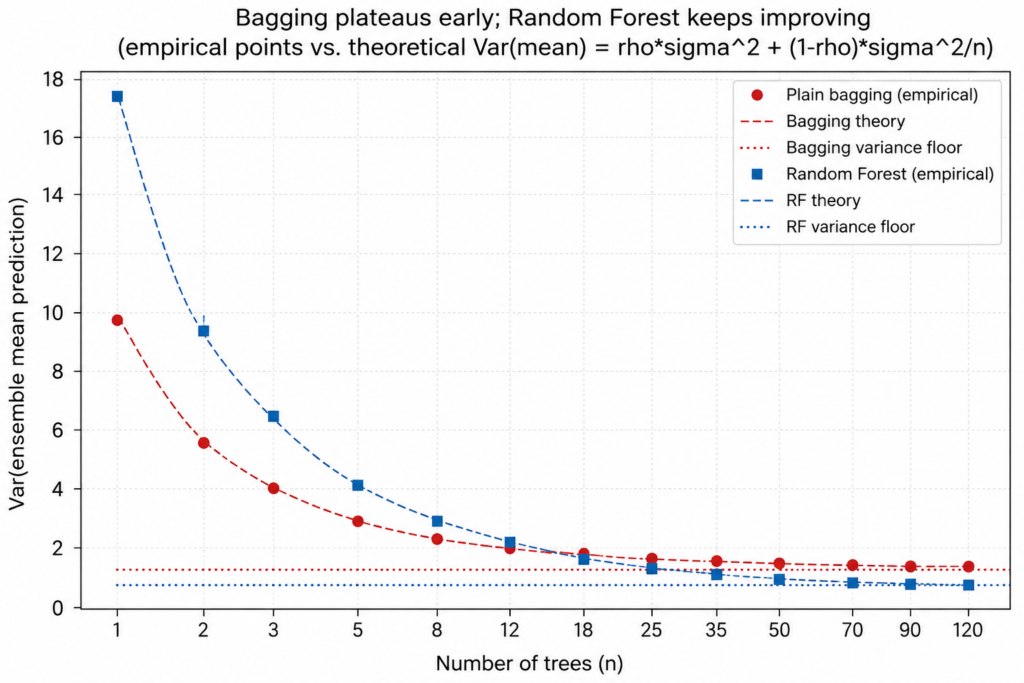The theoretical floor stopped being a symbolic derivation and became a number we can point to and say: this is where it plateaus, and we predicted it.The crossover At n=1, Random Forest starts behind as its lone tree is nearly twice as noisy as bagging’s lone tree (17.42 vs 9.89). But by around n=18, RF has already caught up and overtaken bagging (1.68 vs 1.85). By n=120, RF is sitting at roughly 59% of bagging’s variance (0.85 vs 1.44), despite starting from individually worse building blocks.That crossover is the entire article compressed into one sentence. Averaging alone can’t rescue plain bagging — no matter how many bagged trees you add, you’re stuck above ρσ2≈ρσ² ≈ρσ2≈ 1.34. Random Forest starts from a worse position per tree, but because it decorrelates the ensemble, it keeps improving well past the point where bagging has already flattened out ending up in a completely different neighborhood.All the above can be compressed in the following illustrated image generated by the code in the appendix.The Subtle Point: Worse Trees, Better ForestIt’s worth pausing on something that previous sections numbers already showed, because it’s the detail that surprises people who have used Random Forest for years without digging into why it works: a single Random Forest tree is a strictly worse predictor than a single bagged tree, and yet the Random Forest ensemble ends up strictly better.This isn’t a contradiction but the entire point, once you separate two things that are easy to conflate:Individual quality (how good is one tree, on its own): bagging wins here. σ² = 9.89 for bagging vs 17.42 for RF. Clearly, a bagged tree, seeing all 30 features at every split, simply makes better individual decisions.Ensemble quality (how good is the average of many trees): RF wins here, and not narrowly as at n=120, RF’s ensemble variance is 0.85 vs bagging’s 1.44, roughly 41% lower.The mechanism connecting these is entirely about ρρρ, not σ2σ^2σ2. Feature subsampling doesn’t make trees better — if anything, it makes each one a bit worse, since it’s occasionally forced away from the strongest available split. What it buys is independence between the mistakes different trees make. And because the ensemble variance formula weights ρρρ so heavily (recall: ρρρ survives untouched as n→∞nto inftyn→∞, while σ2σ^2σ2’s contribution shrinks toward zero), a small sacrifice in individual quality can purchase a much larger reduction in shared error.This is a genuinely counter-intuitive trade for anyone used to thinking “better base learner → better ensemble.” For Random Forest specifically, the opposite can hold: a slightly worse base learner, if it’s less correlated with its peers, produces a meaningfully better ensemble. It’s the same logic behind why a portfolio of mediocre, uncorrelated bets can outperform a portfolio of excellent, highly correlated ones; diversification has real value, and it can outweigh individual quality once you’re combining many things.Practical Takeaway: max_features Isn’t a DetailIf there’s one parameter in sklearn.ensemble.RandomForestRegressor (or RandomForestClassifier) that gets set once to ‘sqrt’ and never touched again, it’s max_features. The results above suggest that’s often leaving something on the table.The tradeoff, made concretemax_features controls exactly the quantity this whole article has been about: how many features each split can see, which directly trades off σ2σ²σ2 against ρρρ.Too high (close to, or equal to, all features — i.e. plain bagging): every tree gravitates toward the same dominant features, and you hit the floor early. Adding more trees past that point burns compute for essentially nothing.Too low (e.g. 1 feature per split): trees become so restricted they’re barely better than random guessing at each split, and the floor, while lower in ρρρ terms, can end up higher in absolute Var(mean) terms because σ2σ²σ2 has grown faster than ρρρ shrank.Somewhere between these two extremes is a sweet spot — and where it sits depends on the data, specifically on how many features are genuinely dominant versus how many carry real, if secondary, signal.The one-line mental model to carry forwardmax_features isn’t a randomness dial you set and forget — it’s the lever that decides where your forest sits on the σ2−ρσ² – ρσ2−ρ tradeoff. Tune it the way you would tune any bias-variance knob: by checking what it does to your actual validation error, not by trusting the default because it’s the default.AppendixHere you can find the code I built and used for the analysis. Feel free to execute and reproduce my results or experiment with different parameters. (Estimated time of run ~ 7 mins)”””Bagging vs Random Forest: measuring rho (tree correlation) and thevariance floor Var(mean) = rho*sigma^2 + (1-rho)*sigma^2/n.KEY METHODOLOGICAL POINT:With a FIXED training set, if each tree’s bootstrap sample is drawnindependently, tree predictions are mathematically INDEPENDENT (rho = 0exactly) — this follows from a basic probability fact: if A and B areindependent random variables, then g(A) and h(B) are independent for anyfunctions g, h, even g = h. This holds no matter how nonlinear ordiscontinuous the tree-fitting function is, and despite the fact thatany two bootstrap samples will typically overlap heavily in content –overlap in realized values does not imply statistical dependence.The correlation rho in Breiman’s formula is UNCONDITIONAL: it requiresthe training set itself to be random (drawn from the population) acrossrepeats. All trees in a repeat share that one training-set draw, which isthe actual common source of dependence. So each independent “repeat” ofthis experiment must redraw the training set fresh, not just thebootstrap indices.”””import numpy as npfrom sklearn.tree import DecisionTreeRegressorimport matplotlib.pyplot as pltimport timeRNG_GLOBAL = np.random.default_rng(0)# —————————————————————–# Data-generating process: a couple of DOMINANT features, several# weaker informative features, and pure noise features.# —————————————————————–N_TRAIN = 400N_FEATURES = 30TRUE_COEF = np.zeros(N_FEATURES)TRUE_COEF[0] = 4.0TRUE_COEF[1] = 2.5TRUE_COEF[2:8] = 0.5NOISE_SCALE = 1.5X_PROBE = RNG_GLOBAL.normal(size=(25, N_FEATURES)) # fixed evaluation pointsdef run_repeats(max_features, R, n_max, seed0, max_depth=5): “””R independent repeats. Each repeat: draw a FRESH training set from the population, then train n_max trees on bootstrap resamples of it (with the given max_features policy). Returns predictions at the fixed probe points, shape (R, n_max, n_probe). “”” preds = np.empty((R, n_max, X_PROBE.shape[0])) for r in range(R): rng = np.random.default_rng(seed0 + r) X_train = rng.normal(size=(N_TRAIN, N_FEATURES)) y_train = X_train @ TRUE_COEF + rng.normal(scale=NOISE_SCALE, size=N_TRAIN) for t in range(n_max): idx = rng.integers(0, N_TRAIN, size=N_TRAIN) # bootstrap rows Xb, yb = X_train[idx], y_train[idx] tree = DecisionTreeRegressor( max_features=max_features, # None = bagging, ‘sqrt’ = RF max_depth=max_depth, random_state=rng.integers(0, 1_000_000), ) tree.fit(Xb, yb) preds[r, t, :] = tree.predict(X_PROBE) return predsdef pairwise_rho(preds, n_slots=10): “””Average pairwise correlation between distinct tree ‘slots’, across independent repeats, at fixed test points (unconditional rho, per Breiman’s definition). “”” slots = preds[:, :n_slots, :] rhos = [] for k in range(slots.shape[2]): mat = slots[:, :, k] corr = np.corrcoef(mat, rowvar=False) off = corr.sum() – np.trace(corr) n_pairs = n_slots * (n_slots – 1) rhos.append(off / n_pairs) return float(np.nanmean(rhos))def individual_tree_variance(preds): return float(preds[:, 0, :].var(axis=0).mean())def empirical_var_of_mean(preds, n_values): out = [] for n in n_values: cum_mean = preds[:, :n, :].mean(axis=1) # (R, n_probe) var_per_point = cum_mean.var(axis=0) out.append(float(var_per_point.mean())) return np.array(out)# —————————————————————–# Run the experiment# —————————————————————–R = 400 # independent repeats (reduce to ~100 for a faster run)N_MAX = 120 # max ensemble size probedN_VALUES = np.array([1, 2, 3, 5, 8, 12, 18, 25, 35, 50, 70, 90, 120])t0 = time.time()preds_bag = run_repeats(max_features=None, R=R, n_max=N_MAX, seed0=10_000)t1 = time.time()print(f”Bagging: {t1-t0:.1f}s”)preds_rf = run_repeats(max_features=”sqrt”, R=R, n_max=N_MAX, seed0=50_000)t2 = time.time()print(f”RF: {t2-t1:.1f}s”)rho_bag = pairwise_rho(preds_bag)rho_rf = pairwise_rho(preds_rf)sigma2_bag = individual_tree_variance(preds_bag)sigma2_rf = individual_tree_variance(preds_rf)floor_bag = rho_bag * sigma2_bagfloor_rf = rho_rf * sigma2_rfvar_bag = empirical_var_of_mean(preds_bag, N_VALUES)var_rf = empirical_var_of_mean(preds_rf, N_VALUES)print(f”nrho: bagging={rho_bag:.4f} RF={rho_rf:.4f}”)print(f”sigma^2: bagging={sigma2_bag:.3f} RF={sigma2_rf:.3f}”)print(f”floor: bagging={floor_bag:.3f} RF={floor_rf:.3f}”)print(f”n{‘n’: >5} {‘bag_emp’: >10} {‘bag_theory’: >11} {‘rf_emp’: >10} {‘rf_theory’: >11}”)for n, vb, vr in zip(N_VALUES, var_bag, var_rf): tb = rho_bag * sigma2_bag + (1 – rho_bag) * sigma2_bag / n tr = rho_rf * sigma2_rf + (1 – rho_rf) * sigma2_rf / n print(f”{n: >5} {vb: >10.3f} {tb: >11.3f} {vr: >10.3f} {tr: >11.3f}”)# —————————————————————–# Plot# —————————————————————–fig, ax = plt.subplots(figsize=(9, 6))n_smooth = np.linspace(1, N_VALUES.max(), 300)theory_bag = rho_bag*sigma2_bag + (1-rho_bag)*sigma2_bag/n_smooththeory_rf = rho_rf*sigma2_rf + (1-rho_rf)*sigma2_rf/n_smoothax.plot(N_VALUES, var_bag, “o”, color=”#d62728″, label=”Plain bagging (empirical)”, markersize=6, zorder=5)ax.plot(n_smooth, theory_bag, “–“, color=”#d62728″, alpha=0.6, label=f”Bagging theory (rho={rho_bag:.3f})”)ax.axhline(floor_bag, color=”#d62728″, linestyle=”:”, alpha=0.5, linewidth=1.5)ax.plot(N_VALUES, var_rf, “s”, color=”#1f77b4″, label=”Random Forest (empirical)”, markersize=6, zorder=5)ax.plot(n_smooth, theory_rf, “–“, color=”#1f77b4″, alpha=0.6, label=f”RF theory (rho={rho_rf:.3f})”)ax.axhline(floor_rf, color=”#1f77b4″, linestyle=”:”, alpha=0.5, linewidth=1.5)ax.text(N_VALUES.max()*0.65, floor_bag+0.05, f”bagging floor = rho*sigma^2 = {floor_bag:.2f}”, color=”#d62728″, fontsize=9)ax.text(N_VALUES.max()*0.65, floor_rf+0.05, f”RF floor = rho*sigma^2 = {floor_rf:.2f}”, color=”#1f77b4″, fontsize=9)ax.set_xlabel(“Number of trees (n)”, fontsize=12)ax.set_ylabel(“Var(ensemble mean prediction)”, fontsize=12)ax.set_title(“Bagging plateaus early; Random Forest keeps improvingn” “(empirical points vs. theoretical Var(mean) = rho*sigma^2 + (1-rho)*sigma^2/n)”, fontsize=12)ax.legend(fontsize=9, loc=”upper right”)ax.set_ylim(bottom=0)ax.grid(alpha=0.3)plt.tight_layout()plt.show()References:Breiman, L. (2001). Random Forests. Machine Learning, 45(1), 5–32.